Next: Bibliography
Up: Numerical examples
Previous: Density estimation with Gaussian
Contents
Having seen Bayesian field theoretical models working
for Gaussian prior factors
we will study in this section the
slightly more complex prior mixture models.
Prior mixture models
are an especially useful tool
for implementing complex and
unsharp prior knowledge.
They may be used, for example,
to translate verbal statements of experts
into quantitative prior densities
[132,133,134,135,136],
similar to the
quantification of ``linguistic variables'' by fuzzy methods
[118,119].
We will now study a prior mixture with
Gaussian prior components in  .
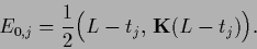
Hence, consider the following energy functional with mixture prior
.
Hence, consider the following energy functional with mixture prior
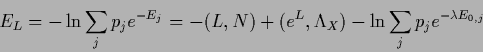 |
(719) |
with mixture components
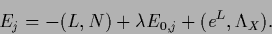 |
(720) |
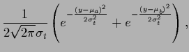
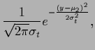
We choose Gaussian component prior factors
with equal covariances but differing means
 |
(721) |
Hence, the stationarity equation for Functional (719)
becomes
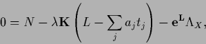 |
(722) |
with Lagrange multiplier function
 |
(723) |
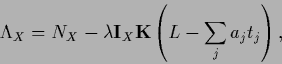
and mixture coefficients
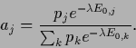 |
(724) |
The parameter  plays here a similar role as the inverse temperature
  for prior mixtures in regression
(see Sect. 6.3).
In contrast to the -parameter in regression, however,
the ``low temperature'' solutions for
for prior mixtures in regression
(see Sect. 6.3).
In contrast to the -parameter in regression, however,
the ``low temperature'' solutions for
 are the pure prior templates
  ,
and for
,
and for
 the prior factor is switched off.
Typical numerical results of a prior mixture model
with two mixture components
are presented in Figs. 23 - 28.
Like for Fig. 21, the true likelihood
used for these calculations is given by Eq. (714)
and shown in Fig. 18.
The corresponding true regression function
is thus that of Fig. 19.
Also, the same training data
have been used as for the model of Fig. 21
(Fig. 20).
The two templates  and
and  which have been selected for the two prior mixture components
are (Fig. 18)
which have been selected for the two prior mixture components
are (Fig. 18)
with
 =
=  ,
,
 =
=  =
=  ,
,
 =
=  =
=  ,
and
,
and  =
=  .
Both templates capture a bit of the structure of the true likelihood,
but not too much, so learning remains interesting.
The average test error of is equal to 2.56
and is thus lower than that of being equal to 2.90.
The minimal possible average test error 2.23
is given by that of the true solution
.
Both templates capture a bit of the structure of the true likelihood,
but not too much, so learning remains interesting.
The average test error of is equal to 2.56
and is thus lower than that of being equal to 2.90.
The minimal possible average test error 2.23
is given by that of the true solution  .
A uniform
.
A uniform  , being the effective template in
the zero mean case of Fig. 21,
has with 2.68 an average test error
between the two templates and .
, being the effective template in
the zero mean case of Fig. 21,
has with 2.68 an average test error
between the two templates and .
Fig. 23 proves
that convergence is fast for massive prior relaxation
when starting from as initial guess  .
Compared to Fig. 21 the solution is a bit smoother,
and as template is a better reference than the uniform likelihood
the final test error is slightly
lower than for the zero-mean Gaussian prior on .
Starting from =
convergence is not much slower
and the final solution is similar,
the test error being in that particular case even lower
(Fig. 24).
Starting from a uniform
the mixture model produces a solution very similar
to that of Fig. 21 (Fig. 25).
.
Compared to Fig. 21 the solution is a bit smoother,
and as template is a better reference than the uniform likelihood
the final test error is slightly
lower than for the zero-mean Gaussian prior on .
Starting from =
convergence is not much slower
and the final solution is similar,
the test error being in that particular case even lower
(Fig. 24).
Starting from a uniform
the mixture model produces a solution very similar
to that of Fig. 21 (Fig. 25).
The effect of changing the
parameter of the prior mixture
can be seen in
Fig. 26
and Fig. 27.
Larger
means a smoother solution
and faster convergence
when starting from a template likelihood
(Fig. 26).
Smaller
results in a more rugged solution
combined with a slower convergence.
The test error in Fig. 27
already indicates overfitting.
Prior mixture models tend to produce metastable
and approximately stable solutions.
Fig. 28 presents an example
where starting with =
the learning algorithm seems to have produced a stable solution
after a few iterations.
However, iterating long enough
this decays into a solution
with smaller distance to and with lower test error.
Notice that this effect can be prevented by starting
with another initialization,
like for example with =
or a similar initial guess.
We have seen now that, and also how,
learning algorithms for Bayesian field theoretical models
can be implemented.
In this paper, the discussion of numerical aspects
was focussed on general density estimation problems.
Other Bayesian field theoretical models,
e.g., for regression and inverse quantum problems,
have also been proved to be numerically feasible.
Specifically,
prior mixture models for Gaussian regression
are compared
with so-called Landau-Ginzburg models
in [132].
An application of prior mixture models
to image completion,
formulated as a Gaussian regression model,
can be found in [137].
Furthermore, hyperparameter have been included in numerical calculations
in [133] and also in [137].
Finally, learning algorithms for
inverse quantum problems are treated
in [143] for inverse quantum statistics,
and, in combination with a mean field approach,
in [142] for inverse quantum many-body theory.
Time-dependent inverse quantum problems
will be the topic of [138].
In conclusion, we may say that
many different Bayesian field theoretical models
have already been studied numerically
and proved to be computationally feasible.
This also shows that such nonparametric Bayesian approaches
are relatively easy to adapt
to a variety of quite different learning scenarios.
Applications of Bayesian field theory
requiring further studies
include, for example, the prediction of time-series
and the interactive implementation of unsharp
a priori information.
Figure 14:
Density estimation with 2 data points
and a Gaussian prior factor
for the log-probability .
First row: Final and .
Second row: The l.h.s. shows the energy  (108)
during iteration,
the r.h.s. the
regression function
(108)
during iteration,
the r.h.s. the
regression function
 =
=
 =
=
 .
The dotted lines indicate the range of
one standard deviation above and below the regression function
(ignoring periodicity in
.
The dotted lines indicate the range of
one standard deviation above and below the regression function
(ignoring periodicity in  ).
The fast convergence shows that the problem is nearly linear.
The asymmetry of the solution
between the - and
).
The fast convergence shows that the problem is nearly linear.
The asymmetry of the solution
between the - and  -direction
is due to the normalization constraint, only required for .
(Laplacian smoothness prior
-direction
is due to the normalization constraint, only required for .
(Laplacian smoothness prior  as given in Eq. (705)
with
as given in Eq. (705)
with
 =
=
 = 1,
= 1,
 = 0,
= 0,
 = 0.025,
 =
=
 = 0.
Iteration with
negative Hessian
= 0.
Iteration with
negative Hessian  =
=  if positive definite,
otherwise with the gradient algorithm, i.e., =
if positive definite,
otherwise with the gradient algorithm, i.e., =  .
Initialization with =
.
Initialization with =
 ,
i.e., normalized to
,
i.e., normalized to
 =
=  ,
with
,
with
 of Eq. (698) and
 =
=
 ,
,  =
=  .
Within each iteration step the optimal step width
.
Within each iteration step the optimal step width  has been found
by a line search.
Mesh with
has been found
by a line search.
Mesh with  points in -direction and
 points in -direction,
periodic boundary conditions in and .
The data points are
points in -direction,
periodic boundary conditions in and .
The data points are  and
and  .)
.)
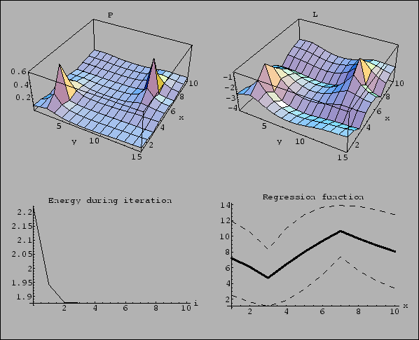 |
Figure 15:
Density estimation with 2 data points,
this time with a Gaussian prior factor
for the probability ,
minimizing the energy functional  (164).
To make the figure comparable with Fig. 14
the parameters have been chosen so that
the maximum of the solution
is the same in both figures (
(164).
To make the figure comparable with Fig. 14
the parameters have been chosen so that
the maximum of the solution
is the same in both figures ( = 0.6).
Notice, that compared to Fig. 14
the smoothness prior is less effective
for small probabilities.
(Same data, mesh
and periodic boundary conditions
as for Fig. 14.
Laplacian smoothness prior
as in Eq. (705)
with
=
= 1,
= 0,
= 1,
=
= 0.
Iterated using massive prior relaxation, i.e.,
=
= 0.6).
Notice, that compared to Fig. 14
the smoothness prior is less effective
for small probabilities.
(Same data, mesh
and periodic boundary conditions
as for Fig. 14.
Laplacian smoothness prior
as in Eq. (705)
with
=
= 1,
= 0,
= 1,
=
= 0.
Iterated using massive prior relaxation, i.e.,
=
 with
with  = 1.0.
Initialization with
= 1.0.
Initialization with  =
=
 ,
with
of Eq. (698)
so is correctly normalized,
and =
,
=
,
with
of Eq. (698)
so is correctly normalized,
and =
,
=  .
Within each iteration step the optimal factor has been found
by a line search algorithm.)
.
Within each iteration step the optimal factor has been found
by a line search algorithm.)
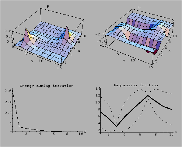 |
Figure 16:
Density estimation with a  Gaussian prior factor
for the log-probability .
Such a prior favors probabilities of Gaussian shape.
(Smoothness prior
of the form of Eq. (705)
with
=
= 1,
= 0,
= 0,
= 0,
= 0.01.
Same iteration procedure, initialization, data, mesh
and periodic boundary conditions
as for Fig. 14.)
Gaussian prior factor
for the log-probability .
Such a prior favors probabilities of Gaussian shape.
(Smoothness prior
of the form of Eq. (705)
with
=
= 1,
= 0,
= 0,
= 0,
= 0.01.
Same iteration procedure, initialization, data, mesh
and periodic boundary conditions
as for Fig. 14.)
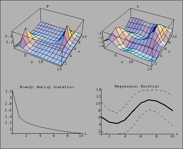 |
Figure 17:
Density estimation with a Gaussian prior factor
for the probability .
As the variation of is smaller than that of ,
a smaller has been chosen than in Fig. 17.
The Gaussian prior in is also relatively less effective
for small probabilities than a comparable Gaussian prior in .
(Smoothness prior
of the form of Eq. (705)
with
=
= 1,
= 0,
= 0,
= 0,
= 0.1.
Same iteration procedure, initialization, data, mesh
and periodic boundary conditions
as for Fig. 15.)
 |
Figure 18:
First row:
True density  (l.h.s.)
true log-density
(l.h.s.)
true log-density  =
=
 (r.h.s.)
used for Figs. 21-28.
Second and third row:
The two templates and
of Figs. 23-28
for (
(r.h.s.)
used for Figs. 21-28.
Second and third row:
The two templates and
of Figs. 23-28
for ( , l.h.s.)
or for (
, l.h.s.)
or for ( , r.h.s.), respectively,
with =
, r.h.s.), respectively,
with =  .
As reference for the following figures
we give the expected test error
.
As reference for the following figures
we give the expected test error
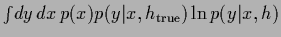 under the true
 for uniform
  .
It is for
.
It is for  equal to 2.23
for template equal to 2.56,
for template equal 2.90
and for a uniform equal to 2.68.
equal to 2.23
for template equal to 2.56,
for template equal 2.90
and for a uniform equal to 2.68.
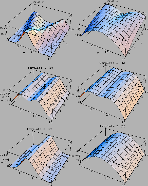 |
Figure 19:
Regression function
 for the true density
of Fig. 18,
defined as
=
=
.
The dashed lines indicate the range of
one standard deviation above and below the regression function.
for the true density
of Fig. 18,
defined as
=
=
.
The dashed lines indicate the range of
one standard deviation above and below the regression function.
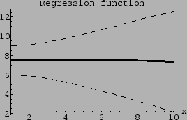 |
Figure 20:
L.h.s.:
Empirical density
 =
=
 .
sampled from
.
sampled from
 =
=
 with uniform .
R.h.s.:
Corresponding conditional empirical density
with uniform .
R.h.s.:
Corresponding conditional empirical density
 =
=
 =
=
 .
Both densities are obtained from the 50 data points
used for Figs. 21-28.
.
Both densities are obtained from the 50 data points
used for Figs. 21-28.
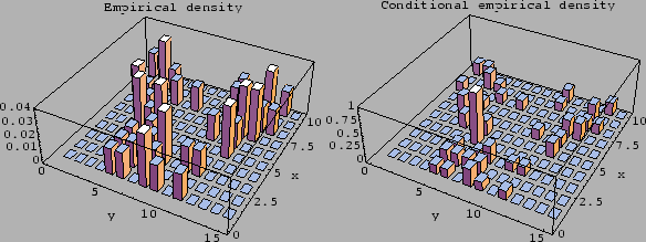 |
Figure 21:
Density estimation with Gaussian prior factor
for log-probability with 50 data points
shown in Fig. 20.
Top row: Final solution  =
=  and
and  .
Second row: Energy (108)
during iteration and final regression function.
Bottom row:
Average training error
.
Second row: Energy (108)
during iteration and final regression function.
Bottom row:
Average training error
 during iteration
and
average test error
during iteration
and
average test error
 for uniform .
(Parameters: Zero mean Gaussian
smoothness prior with
inverse covariance
for uniform .
(Parameters: Zero mean Gaussian
smoothness prior with
inverse covariance
 ,
= 0.5
and
of the form (705)
with
= 2,
= 1,
= 0,
= 1,
=
= 0,
massive prior iteration with
=
and squared mass =
,
= 0.5
and
of the form (705)
with
= 2,
= 1,
= 0,
= 1,
=
= 0,
massive prior iteration with
=
and squared mass =  .
Initialized with normalized constant .
At each iteration step the factor
has been adapted by a line search algorithm.
Mesh with points in -direction and
points in -direction,
periodic boundary conditions in .)
.
Initialized with normalized constant .
At each iteration step the factor
has been adapted by a line search algorithm.
Mesh with points in -direction and
points in -direction,
periodic boundary conditions in .)
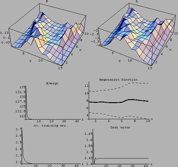 |
Figure 22:
Comparison of iteration schemes and initialization.
First row: Massive prior iteration
(with =
, = )
and uniform initialization.
Second row: Hessian iteration ( = )
and uniform initialization.
Third row: Hessian iteration and kernel initialization
(with =
 , =
and normalized afterwards).
Forth row: Gradient ( = ) with uniform initialization.
Fifth row: Gradient with kernel initialization.
Sixth row: Gradient
with delta-peak initialization.
(Initial equal to
, =
and normalized afterwards).
Forth row: Gradient ( = ) with uniform initialization.
Fifth row: Gradient with kernel initialization.
Sixth row: Gradient
with delta-peak initialization.
(Initial equal to
 ,
,  =
=  ,
conditionally normalized.
For
,
conditionally normalized.
For  see Fig. 20).
Minimal number of iterations 4,
maximal number of iterations 50,
iteration stopped if
see Fig. 20).
Minimal number of iterations 4,
maximal number of iterations 50,
iteration stopped if
 .
Energy functional and parameters as for Fig. 21.
.
Energy functional and parameters as for Fig. 21.
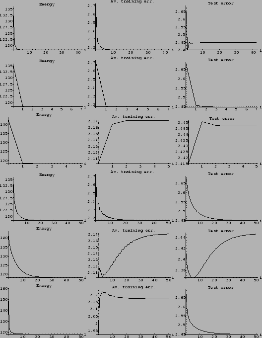 |
Figure 23:
Density estimation with a Gaussian mixture prior
for log-probability
with 50 data points, Laplacian prior and the two template functions
shown in Fig. 18.
Top row: Final solution = and .
Second row: Energy Energy (719)
during iteration and final regression function.
Bottom row:
Average training error
-
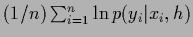 during iteration
and
average test error
for uniform .
(Two mixture components with
= 0.5 and
smoothness prior with
during iteration
and
average test error
for uniform .
(Two mixture components with
= 0.5 and
smoothness prior with  =
=  of the form (705)
with
= 2,
= 1,
= 0,
= 1,
=
= 0,
massive prior iteration with
=
and squared mass = ,
initialized with = .
At each iteration step the factor
has been adapted by a line search algorithm.
Mesh with
of the form (705)
with
= 2,
= 1,
= 0,
= 1,
=
= 0,
massive prior iteration with
=
and squared mass = ,
initialized with = .
At each iteration step the factor
has been adapted by a line search algorithm.
Mesh with  = points in -direction and
 = points in -direction,
 = data points at , ,
periodic boundary conditions in .
Except for the inclusion of two mixture components
parameters are equal to those for Fig. 21. )
= data points at , ,
periodic boundary conditions in .
Except for the inclusion of two mixture components
parameters are equal to those for Fig. 21. )
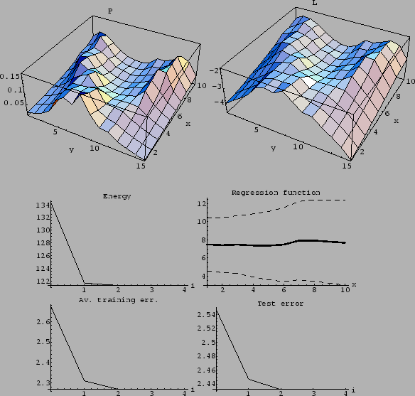 |
Figure 24:
Using a different starting point.
(Same parameters as for Fig. 23,
but initialized with = .)
While the initial guess is worse
then that of Fig. 23,
the final solution is even slightly better.
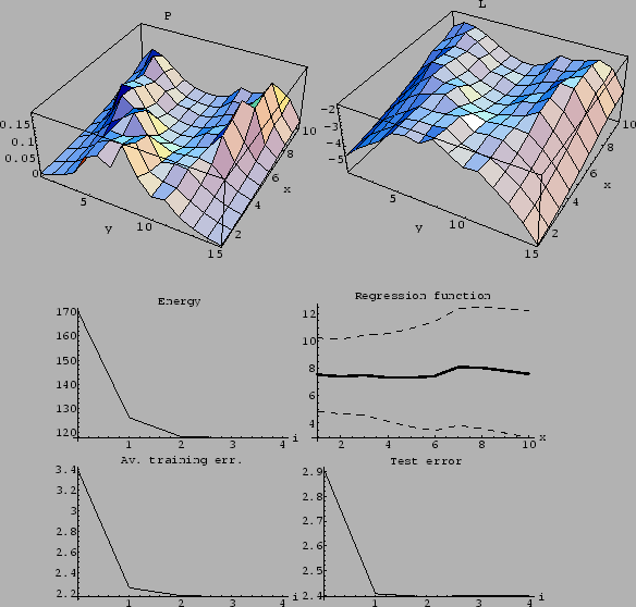 |
Figure 25:
Starting from a uniform initial guess.
(Same as Fig. 23,
but initialized with uniform .)
The resulting solution is, compared to
Figs. 23 and 24,
a bit more wiggly, i.e., more data oriented.
One recognizes a slight ``overfitting'',
meaning that the test error increases
while the training error is decreasing.
(Despite the increasing of the test error during iteration
at this value of ,
a better solution cannot necessarily be found
by just changing -value.
This situation can for example occur, if
the initial guess is better then the implemented prior.)
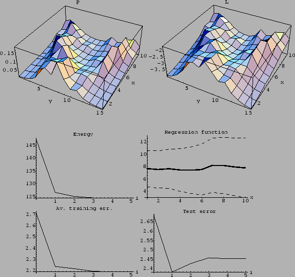 |
Figure 26:
Large .
(Same parameters as for Fig. 23,
except for = 1.0.)
Due to the larger smoothness constraint
the averaged training error is larger than in Fig. 23.
The fact that also the test error is larger than in Fig. 23
indicates that the value of is too large.
Convergence, however, is very fast.
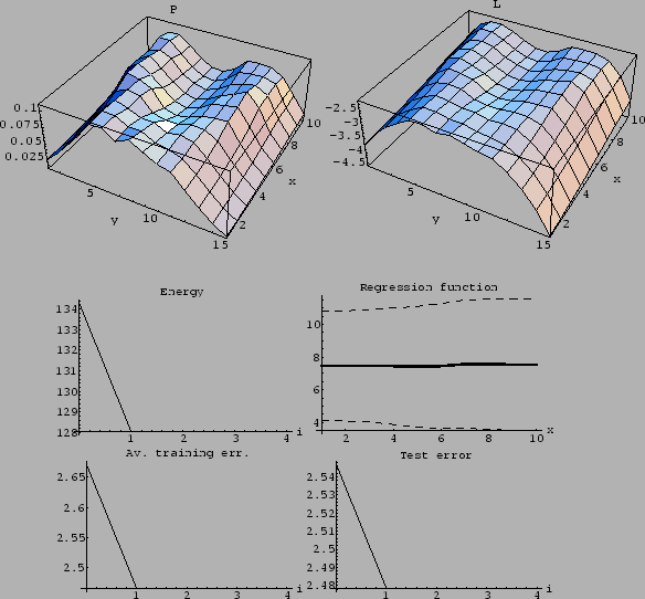 |
Figure 27:
Overfitting due to too small .
(Same parameters as for Fig. 23,
except for = 0.1.)
A small allows the average training error
to become quite small.
However, the average test error grows
already after two iterations.
(Having found at some -value
during iteration an increasing test error,
it is often but not necessarily the case that
a better solution can be found
by changing .)
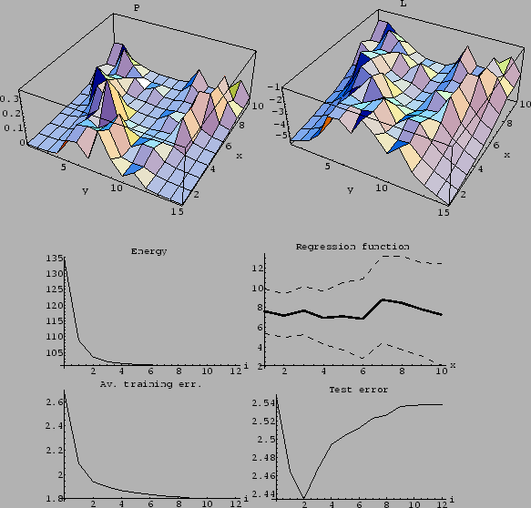 |
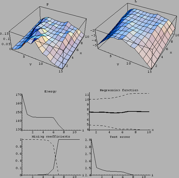
Figure 28:
Example of an approximately stable solution.
(Same parameters as for Fig. 23,
except for =  , =
, =  ,
and initialized with = .)
A nearly stable solution is obtained
after two iterations,
followed by a plateau between iterations 2 and 6.
A better solution is finally found
with smaller distance to template .
(The plateau gets elongated with growing mass
,
and initialized with = .)
A nearly stable solution is obtained
after two iterations,
followed by a plateau between iterations 2 and 6.
A better solution is finally found
with smaller distance to template .
(The plateau gets elongated with growing mass  .)
The figure on the l.h.s. in the bottom row
shows the mixing coefficients
.)
The figure on the l.h.s. in the bottom row
shows the mixing coefficients  of the components of the prior mixture model
for the solution during iteration
(
of the components of the prior mixture model
for the solution during iteration
( , line and
  , dashed).
 |
Acknowledgements
The author wants to thank
Federico Girosi, Tomaso Poggio,
Jörg Uhlig, and Achim Weiguny
for discussions.
Next: Bibliography
Up: Numerical examples
Previous: Density estimation with Gaussian
Contents
Joerg_Lemm
2001-01-21