Next: High and low temperature
Up: Non-Gaussian prior factors
Previous: Prior mixtures for density
Contents
Prior mixtures for regression
For regression it is especially useful to introduce
an inverse temperature multiplying the terms
depending on  , i.e., likelihood and prior.4As in regression is represented by the regression function
  the temperature-dependent error functional becomes
 |
(544) |
with
 |
(545) |
 |
(546) |
some hyperprior energy
 ,
and
,
and
with some constant  .
If we also maximize with respect to
.
If we also maximize with respect to  we have to include the (
 -independent)
training data variance
-independent)
training data variance
 where
where
 =
=
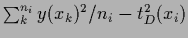 is the variance of the
  training data at
  .
In case every appears only once
.
In case every appears only once  vanishes.
Notice that
vanishes.
Notice that  includes a contribution from the
  data points
arising from the -dependent normalization
of the likelihood term.
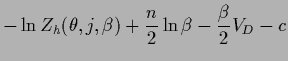
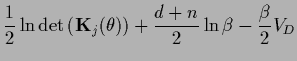
Writing the stationarity equation
for the hyperparameter separately,
the corresponding three stationarity conditions
are found as
data points
arising from the -dependent normalization
of the likelihood term.
Writing the stationarity equation
for the hyperparameter separately,
the corresponding three stationarity conditions
are found as
As is only a one-dimensional parameter
and its density can be quite non-Gaussian
it is probably most times more informative
to solve for varying values of
instead to restrict to a single
`optimal'  .
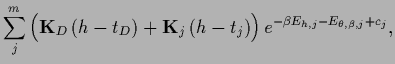
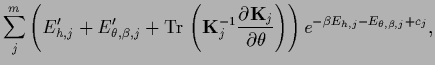
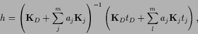
Eq. (548)
can also be written
.
Eq. (548)
can also be written
 |
(551) |
with
being thus still a nonlinear equation for .
Subsections
Next: High and low temperature
Up: Non-Gaussian prior factors
Previous: Prior mixtures for density
Contents
Joerg_Lemm
2001-01-21