Next: Local mixtures
Up: Prior mixtures for regression
Previous: Equal covariances
Contents
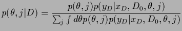
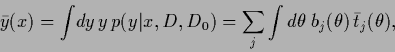
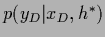
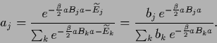
For regression under a Gaussian mixture model
the predictive density can be calculated analytically
for fixed  .
The predictive density can be expressed
in terms of the likelihood of
and
.
The predictive density can be expressed
in terms of the likelihood of
and  ,
marginalized over
,
marginalized over  ,
,
 |
(576) |
(Here we concentrate on .
The parameter  can be treated analogously.)
According to Eq. (492) the likelihood can be written
can be treated analogously.)
According to Eq. (492) the likelihood can be written
 |
(577) |
with
 |
(578) |
and
 =
=
 being a
 -matrix in data space.
The equality of
-matrix in data space.
The equality of  and
and
 can be seen using
 =
=
 =
=
 =
=
 .
For the predictive mean,
being the optimal solution under squared-error loss
and log-loss (restricted to Gaussian densities with fixed variance)
we find therefore
.
For the predictive mean,
being the optimal solution under squared-error loss
and log-loss (restricted to Gaussian densities with fixed variance)
we find therefore
 |
(579) |
with, according to Eq. (327),
 |
(580) |
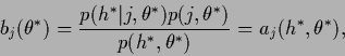
and mixture coefficients
which defines
 =
=
 +
+  .
For solvable -integral
the coefficients can therefore be obtained exactly.
.
For solvable -integral
the coefficients can therefore be obtained exactly.
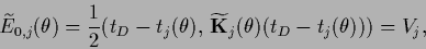
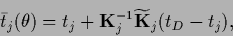
If  is calculated in saddle point
approximation at =
is calculated in saddle point
approximation at =  it has the structure of
  in (552)
with
in (552)
with  replaced by
and
replaced by
and
 by
by
 .
(The inverse temperature could be treated analogously to .
In that case would have to be replaced by
.
(The inverse temperature could be treated analogously to .
In that case would have to be replaced by
 .)
.)
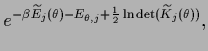
Calculating also the likelihood for ,
in Eq. (581)
in saddle point approximation, i.e.,
 ,
the terms
,
the terms
 in numerator and denominator cancel,
so that, skipping
in numerator and denominator cancel,
so that, skipping  and ,
and ,
 |
(582) |
becomes equal to
the  in Eq. (552) at
=
in Eq. (552) at
=  .
.
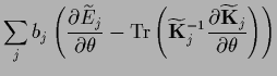
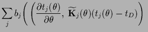
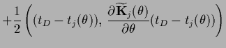
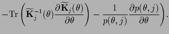
Eq. (581) yields
as stationarity equation for ,
similarly to Eq. (494)
For fixed and -independent covariances
the high temperature solution
is a mixture of component solutions
weighted by their prior probability
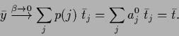 |
(585) |
The low temperature solution becomes the
component solution  with minimal
distance between data and prior template
with minimal
distance between data and prior template
 |
(586) |
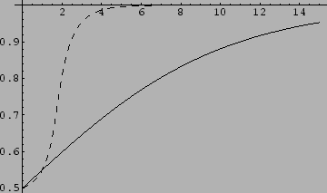
Fig.11 compares
the exact mixture coefficient  with the dominant solution of the maximum
posterior coefficient
with the dominant solution of the maximum
posterior coefficient  (see also [132])
which are related according to (569)
(see also [132])
which are related according to (569)
 |
(587) |
Figure 11:
Exact and (dashed) vs.
for two mixture components with equal covariances
and  =
=  = 2,
= 2,
 = 0.405,
 = 0.605.
 |
Next: Local mixtures
Up: Prior mixtures for regression
Previous: Equal covariances
Contents
Joerg_Lemm
2001-01-21