Next: Analytical solution of mixture
Up: Prior mixtures for regression
Previous: High and low temperature
Contents
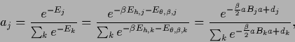
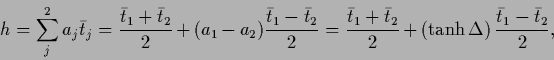
Especially interesting is the case
of  -independent
 =
=
 and
and  -independent
 .
In that case the often difficult to obtain
determinants of
.
In that case the often difficult to obtain
determinants of  do not have to be calculated.
For -independent inverse covariances
the high temperature solution
is
according to
Eqs.(555,561)
a linear combination
of the (potential) low temperature solutions
 |
(566) |
It is worth to emphasize that, as the solution
 is not a mixture of the component templates
  but of component solutions
  ,
even poor choices for the template functions
can lead to good solutions, if enough data are available.
That is indeed the reason why the most common choice
,
even poor choices for the template functions
can lead to good solutions, if enough data are available.
That is indeed the reason why the most common choice  for a Gaussian prior can be successful.
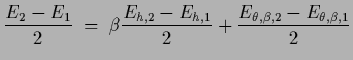
Eqs.(565) simplifies to
 |
(567) |
where
 |
(568) |
and (for -independent  )
)
 |
(569) |
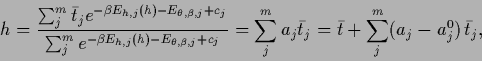
introducing
vector  with components
  ,
,
 matrices
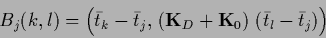 |
(570) |
and constants
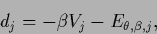 |
(571) |
with  given in (564).
Eq. (567) is still a nonlinear equation
for
given in (564).
Eq. (567) is still a nonlinear equation
for  , it shows however that the solutions
must be convex combinations of the -independent .
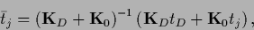
Thus, it is sufficient to solve
Eq. (569) for
, it shows however that the solutions
must be convex combinations of the -independent .
Thus, it is sufficient to solve
Eq. (569) for  mixture coefficients
instead of Eq. (548) for the function .
mixture coefficients
instead of Eq. (548) for the function .
The high temperature relation
Eq. (553) becomes
 |
(572) |
or  for a hyperprior
 uniform with respect to .
The low temperature relation Eq. (559)
remains unchanged.
uniform with respect to .
The low temperature relation Eq. (559)
remains unchanged.
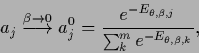
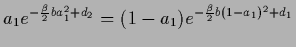
For  Eq. (567) becomes
 |
(573) |
with
 =
in case
=
in case
 is uniform in
so that
is uniform in
so that  =
=  , and
, and
because
the matrices  are in this case zero except
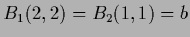 .
The stationarity Eq. (569) can be solved
graphically (see Figs.7, 8),
the solution being given by the point
where
.
The stationarity Eq. (569) can be solved
graphically (see Figs.7, 8),
the solution being given by the point
where
 ,
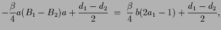
or, alternatively,
,
or, alternatively,
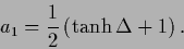 |
(575) |
That equation is analogous to
the celebrated mean field equation of the
ferromagnet.
We conclude that in the case of equal component covariances,
in addition to the linear low-temperature equations,
only a  -dimensional nonlinear equation has to be solved
to determine the
`mixing coefficients'
-dimensional nonlinear equation has to be solved
to determine the
`mixing coefficients'
 .
.
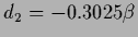
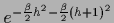
Figure:
The solution of stationary equation
Eq. (569) is given by the point where
 =
=
 (upper row) or, equivalently,
 =
=
 (lower row).
Shown are, from left to right, a situation
at high temperature and one stable solution (
(lower row).
Shown are, from left to right, a situation
at high temperature and one stable solution ( =
=  ),
at a temperature ( =
),
at a temperature ( =  ) near the bifurcation,
and at low temperature with
two stable and one unstable solutions =
) near the bifurcation,
and at low temperature with
two stable and one unstable solutions =  .
The values of
.
The values of  = ,
= ,
 and
and
 used for the plots
correspond for example to the one-dimensional
model of Fig.9 with
used for the plots
correspond for example to the one-dimensional
model of Fig.9 with  ,
,  ,
,  .
Notice, however, that the shown relation is valid
for at arbitrary dimension.
.
Notice, however, that the shown relation is valid
for at arbitrary dimension.
 |
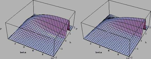
Figure 8:
As in Fig.7
the plots of  and
and
 are shown
within the inverse temperature range
are shown
within the inverse temperature range
 .
.
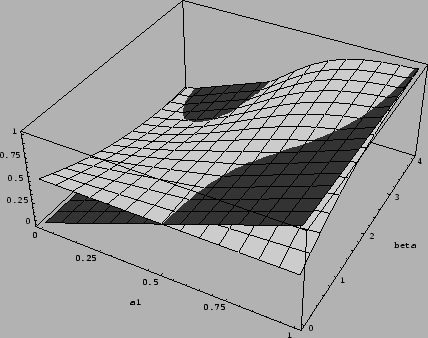 |
Figure 9:
Shown is the joint posterior density of  and , i.e.,
 for a zero-dimensional example
of a Gaussian prior mixture model
with training data
for a zero-dimensional example
of a Gaussian prior mixture model
with training data  and prior data
  and inverse temperature .
L.h.s.:
For uniform prior (middle)
and inverse temperature .
L.h.s.:
For uniform prior (middle)
 with
joint posterior
with
joint posterior 

 the maximum appears at finite .
(Here no factor
the maximum appears at finite .
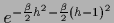
(Here no factor  appears in front of
  because normalization constants for prior and likelihood term have
to be included.)
R.h.s.:
For compensating hyperprior
because normalization constants for prior and likelihood term have
to be included.)
R.h.s.:
For compensating hyperprior
 with
with

 the maximum is at =
  .
.
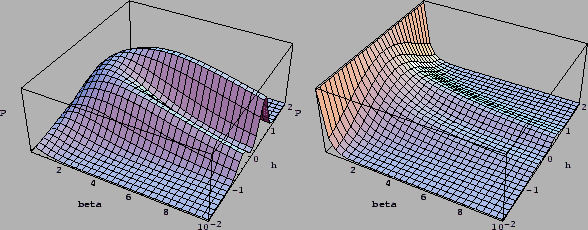 |
Figure 10:
Same zero-dimensional prior mixture model
for uniform hyperprior on
as in Fig.9,
but for varying data
 (left),
 (right).
 |
Next: Analytical solution of mixture
Up: Prior mixtures for regression
Previous: High and low temperature
Contents
Joerg_Lemm
2001-01-21