Lagrange multipliers: Error functional $E_L$

In this chapter we look at density estimation problems with Gaussian prior factors. We begin with a discussion of functional priors which are Gaussian in probabilities or in log-probabilities, and continue with general Gaussian prior factors. Two sections are devoted to the discussion of covariances and means of Gaussian prior factors, as their adequate choice is essential for practical applications. After exploring some relations of Bayesian field theory and empirical risk minimization, the last three sections introduce the specific likelihood models of regression, classification, inverse quantum theory.

We begin with a discussion of Gaussian prior factors in $L$. As Gaussian prior factors correspond to quadratic error (or energy) terms, consider an error functional with a quadratic regularizer in $L$

$$(L,{{\bf K}}L)=\vert\vert L\vert\vert^2_{{\bf K}} = \frac{1}... ...x,y) {{\bf K}}(x,y;x^\prime,y^\prime ) L(x^\prime ,y^\prime) ,$$ (106)

writing for the sake of simplicity from now on $L(x,y)$ for the log-probability $L(y\vert x,{h})$ = $\ln p(y\vert x,{h})$. The operator ${{\bf K}}$ is assumed symmetric and positive semi-definite and positive definite on some subspace. (We will understand positive semi-definite to include symmetry in the following.) For positive (semi-)definite ${{\bf K}}$ the scalar product defines a (semi-)norm by

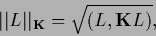$$\vert\vert L\vert\vert _{{\bf K}} = \sqrt{(L,{{\bf K}}L)} ,$$ (107)

and a corresponding distance by $\vert\vert L-L^\prime\vert\vert _{{\bf K}}$. The quadratic error term (106) corresponds to a Gaussian factor of the prior density which have been called the specific prior $p({h}\vert\tilde D_0)$ = $p(L\vert\tilde D_0)$ for $L$. In particular, we will consider here the posterior density

$$p({h}\vert f) \! \propto e^{ \sum_i L_i(x_i,y_i) - \!\frac{... ... (x) \left( 1 - \int\!dy\, e^{L(x,y)} \right) + \tilde c, } ,$$ (108)

where prefactors like $\beta$ are understood to be included in ${{\bf K}}$. The constant $\tilde c$ referring to the specific prior is determined by the determinant of ${{\bf K}}$ according to Eq. (70). Notice however that not only the likelihood $\sum_i L_i$ but also the complete prior is usually not Gaussian due to the presence of the normalization conditions. (An exception is Gaussian regression, see Section 3.7.) The posterior (108) corresponds to an error functional

$$E_L = \beta E_{\rm comb} = -(L,N) + \frac{1}{2} (L,{{\bf K}} L) +(e^L-\delta(y),\Lambda_X) ,$$ (109)

with likelihood vector (or function)

$$L(x,y) = L(y\vert x,{h}) ,$$ (110)

data vector (function)

$$N(x,y) = \sum_i^n \delta(x-x_i)\delta(y-y_i) ,$$ (111)

Lagrange multiplier vector (function)

$$\Lambda_X(x,y) = \Lambda_X(x) ,$$ (112)

probability vector (function)

$$e^L(x,y) = e^{L(x,y)} = P(x,y) = p(y\vert x,{h}) ,$$ (113)

and

$$\delta(y)(x,y) =\delta(y) .$$ (114)

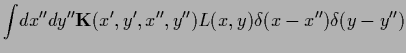
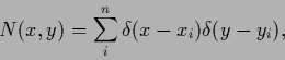
According to Eq. (111) $N/n$ = $P_{\rm emp}$ is an empirical density function for the joint probability $p(x,y\vert{h})$.

We end this subsection by defining some notations. Functions of vectors (functions) and matrices (operators), different from multiplication, will be understood element-wise like for example $(e^L)(x,y)$ = $e^{L(x,y)}$. Only multiplication of matrices (operators) will be interpreted as matrix product. Element-wise multiplication has then to be written with the help of diagonal matrices. For that purpose we introduce diagonal matrices made from vectors (functions) and denoted by the corresponding bold letters. For instance,

$${\bf I} (x,y ; x^\prime,y^\prime) = \delta (x-x^\prime) \delta (y-y^\prime),$$ (115)

$${\bf L} (x,y;x^\prime,y^\prime ) = \delta (x-x^\prime)\delta (y-y^\prime) L(x,y),$$ (116)

$${\bf P} (x,y;x^\prime,y^\prime ) = {\bf e^L} (x,y;x^\prime,y^\prime )$$ (117)

$$= \delta (x-x^\prime)\delta (y-y^\prime) P(x,y),$$ (118)

$${\bf N} (x,y ; x^\prime,y^\prime) = \delta (x-x^\prime) \delta (y-y^\prime) \, N(x,y),$$ (119)

$${\bf\Lambda}_X (x,y;x^\prime,y^\prime ) = \delta (x-x^\prime)\delta (y-y^\prime) \Lambda_X (x) ,$$ (120)

or

$$L = {\bf L} I,\quad P = {\bf P} I,\quad e^L = {\bf e^L} I,\quad N = {\bf N} I,\quad \Lambda_X = {\bf\Lambda}_X I ,$$ (121)

where

$$I(x,y) = 1 .$$ (122)

Being diagonal all these matrices commute with each other. Element-wise multiplication can now be expressed as

$$({{\bf K}} {\bf L}) (x^\prime,y^\prime,x,y) = \int \!dx^{\prime\prime}dy^{\prime\prime} {{\bf K}}(x^\prime,y^\p... ...{\prime\prime},y^{\prime\prime}) {\bf L}(x^{\prime\prime},y^{\prime\prime},x,y)$$

$$= \int \!dx^{\prime\prime}dy^{\prime\prime} {{\bf K}}(x^\prime,y^\p... ...},y^{\prime\prime}) L(x,y) \delta(x-x^{\prime\prime})\delta(y-y^{\prime\prime})$$

$$= {{\bf K}}(x^\prime,y^\prime,x,y) L(x,y) .$$ (123)

In general this is not equal to $L(x^\prime,y^\prime ) {{\bf K}}(x^\prime,y^\prime,x,y)$. In contrast, the matrix product ${{\bf K}} L$ with vector $L$

$$({{\bf K}} L) (x^\prime,y^\prime) = \int \!dx\,dy\,{{\bf K}}(x^\prime,y^\prime,x,y) L(x,y) ,$$ (124)

does not depend on $x$, $y$ anymore, while the tensor product or outer product,

$$({{\bf K}} \otimes L)(x^{\prime\prime},y^{\prime\prime},x,y,... ...\prime\prime},y^{\prime\prime},x^{\prime},y^{\prime}) L(x,y) ,$$ (125)

depends on additional $x^{\prime\prime}$, $y^{\prime\prime}$.

Taking the variational derivative of (108) with respect to $L(x,y)$ using

$$\frac{ \delta L(x^\prime,y^\prime) }{\delta L(x,y )} = \delta (x-x^\prime ) \delta (y-y^\prime )$$ (126)

and setting the gradient equal to zero yields the stationarity equation

$$0 = N - {{\bf K}} L - {\bf e^L} \Lambda_X .$$ (127)

Alternatively, we can write ${\bf e^L} \Lambda_X$ = ${\bf\Lambda}_X e^L$ = ${\bf P} \Lambda_X$.

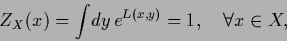
The Lagrange multiplier function $\Lambda_X$ is determined by the normalization condition

$$Z_X(x) = \int \!dy \, e^{L(x,y)} = 1, \quad \forall x\in X ,$$ (128)

which can also be written

$$Z_X = {\bf I}_X P = {\bf I}_X e^L = I \quad \mbox{\rm or} \quad {\bf Z}_X = {\bf I},$$ (129)

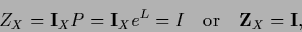
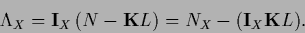
in terms of normalization vector,

$$Z_X(x,y) = Z_X(x) ,$$ (130)

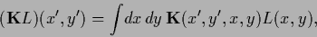
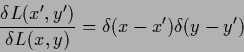
normalization matrix,

$${\bf Z_X} (x,y ; x^\prime,y^\prime) =\delta (x-x^\prime) \delta (y-y^\prime) \, Z_X(x) ,$$ (131)

and identity on $X$,

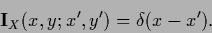$${\bf I}_X (x,y;x^\prime,y^\prime) = \delta(x-x^\prime) .$$ (132)

Multiplication of a vector with ${\bf I}_X$ corresponds to $y$-integration. Being a non-diagonal matrix ${\bf I}_X$ does in general not commute with diagonal matrices like ${\bf L}$ or ${\bf P}$. Note also that despite ${\bf I}_X e^L$ = ${\bf I}_X {\bf e^L} I$ = ${\bf I}I$ = $I$ in general ${\bf I}_X {\bf P}$ = ${\bf I}_X {\bf e^L}\ne {\bf I}$ = ${\bf Z}_X$. According to the fact that ${\bf I}_X$ and ${\bf\Lambda}_X$ commute, i.e.,

$${\bf I}_X {\bf\Lambda}_X ={\bf\Lambda}_X {\bf I}_X \Leftrig... ... = {\bf\Lambda}_X {\bf I}_X - {\bf I}_X {\bf\Lambda}_X = 0 ,$$ (133)

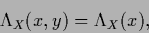
(introducing the commutator $[A,B]$ = $AB-BA$), and that the same holds for the diagonal matrices

$$[{\bf\Lambda}_X , {\bf e^L} ]= [{\bf\Lambda}_X , {\bf P} ] = 0 ,$$ (134)

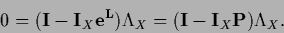
it follows from the normalization condition ${\bf I}_X P$ = $I$ that

$${\bf I}_X {\bf P} \Lambda_X = {\bf I}_X {\bf\Lambda_X} P = {\bf\Lambda_X} {\bf I}_X P = {\bf\Lambda_X} I = \Lambda_X ,$$ (135)

i.e.,

$$0= ({\bf I} - {\bf I}_X {\bf e^L}) \Lambda_X =({\bf I} - {\bf I}_X {\bf P}) \Lambda_X .$$ (136)

For $\Lambda_X(x) \ne 0$ Eqs.(135,136) are equivalent to the normalization (128). If there exist directions at the stationary point $L^*$ in which the normalization of $P$ changes, i.e., the normalization constraint is active, a $\Lambda_X(x) \ne 0$ restricts the gradient to the normalized subspace (Kuhn-Tucker conditions [57,19,99,193]). This will clearly be the case for the unrestricted variations of $p(y,x)$ which we are considering here. Combining $\Lambda_X$ = ${\bf I}_X {\bf P} \Lambda_X$ for $\Lambda_X(x) \ne 0$ with the stationarity equation (127) the Lagrange multiplier function is obtained

$$\Lambda_X = {\bf I}_X \left( N - {{\bf K}} L \right) = N_X - ({\bf I}_X{{\bf K}} L) .$$ (137)

Here we introduced the vector

$$N_X = {\bf I}_X N ,$$ (138)

with components

$$N_X (x,y) = N_X (x) = \sum_i \delta (x - x_i) = n_x ,$$ (139)

giving the number of data available for $x$. Thus, Eq. (137) reads in components

$$\Lambda_X (x) = \sum_i \delta (x - x_i) - \int \! dy^{\prim... ...x,y^{\prime\prime};x^\prime,y^\prime ) L(x^\prime, y^\prime ).$$ (140)

We remark, that for a Laplacian ${\bf K}$ and appropriate boundary conditions the integral term in equation (140) vanishes.

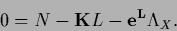
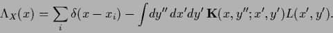
Inserting now the equation (140) for $\Lambda_X$ into the stationarity equation (127) yields

$$0 = N - {{\bf K}} L - {\bf e^L} ( N_X - {\bf I}_X {{\bf K}} ... ... I}-{\bf e^L} {\bf I}_X \right) \left(N- {{\bf K}} L \right) .$$ (141)

Eq. (141) possesses, besides normalized solutions we are looking for, also possibly unnormalized solutions fulfilling $N={{\bf K}}L$ for which Eq. (137) yields $\Lambda_X = 0$. That happens because we used Eq. (135) which is also fulfilled for $\Lambda_X(x) = 0$. Such a $\Lambda_X(x) = 0$ does not play the role of a Lagrange multiplier. For parameterizations of $L$ where the normalization constraint is not necessarily active at a stationary point $\Lambda_X(x) = 0$ can be possible for a normalized solution $L^*$. In that case normalization has to be checked.

It is instructive to define

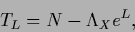$$T_L = N - \Lambda_X e^L ,$$ (142)

so the stationarity equation (127) acquires the form

$${{\bf K}} L = T_L,$$ (143)

which reads in components

$$\int \! dx^\prime dy^\prime \, {{\bf K}} (x,y;x^\prime,y^\pr... ...ta (x-x_i) \delta (y-y_i) - {\bf\Lambda}_X (x) \, e^{L(x,y)} ,$$ (144)

which is in general a non-linear equation because $T_L$ depends on $L$. For existing (and not too ill-conditioned) ${{\bf K}}^{-1}$ the form (143) suggest however an iterative solution of the stationarity equation according to

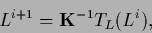$$L^{i+1} = {{\bf K}}^{-1} T_L(L^i) ,$$ (145)

for discretized $L$, starting from an initial guess $L^0$. Here the Lagrange multiplier $\Lambda_X$ has to be adapted so it fulfills condition (137) at the end of iteration. Iteration procedures will be discussed in detail in Section 7.