Next: Normalization, non-negativity, and specific
Up: Bayesian framework
Previous: General loss functions and
Contents
Maximum A Posteriori Approximation
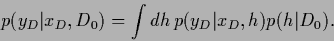
In most applications
the (usually very high or even formally infinite dimensional)
 -integral over model states
in Eq. (23)
cannot be performed exactly.
The two most common methods used to calculate
the integral approximately are
Monte Carlo integration
[155,91,95,198,16,70,199,21,219,238,69,170,180,202,171]
and saddle point approximation
[16,45,30,172,17,249,201,69,76,132].
The latter approach will be studied in the following.
-integral over model states
in Eq. (23)
cannot be performed exactly.
The two most common methods used to calculate
the integral approximately are
Monte Carlo integration
[155,91,95,198,16,70,199,21,219,238,69,170,180,202,171]
and saddle point approximation
[16,45,30,172,17,249,201,69,76,132].
The latter approach will be studied in the following.
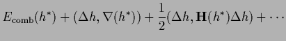
For that purpose, we expand  of Eq. (24)
with respect to around some
of Eq. (24)
with respect to around some 
with
 =
=
 ,
gradient
,
gradient  (not acting on ),
Hessian
(not acting on ),
Hessian  ,
and round brackets
,
and round brackets
 denoting scalar products.
In case
denoting scalar products.
In case  is parameterized independently for
every
is parameterized independently for
every  ,
,  the states represent a parameter set
indexed by and , hence
the states represent a parameter set
indexed by and , hence
 |
(67) |
 |
(68) |
are functional derivatives
[97,106,29,36]
(or partial derivatives for discrete , )
and for example
 |
(69) |
Choosing to be the location of a local minimum
of
 the linear term in (66)
vanishes. The second order term
includes the Hessian
and corresponds to a Gaussian integral over
which could be solved analytically
the linear term in (66)
vanishes. The second order term
includes the Hessian
and corresponds to a Gaussian integral over
which could be solved analytically
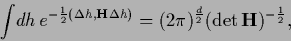 |
(70) |
for a  -dimensional -integral.
However,
using the same approximation for
the -integrals in numerator and denominator of Eq. (23),
expanding then also around ,
and restricting to the first (-independent) term
-dimensional -integral.
However,
using the same approximation for
the -integrals in numerator and denominator of Eq. (23),
expanding then also around ,
and restricting to the first (-independent) term
 of that expansion,
the factor (70) cancels, even for infinite .
(The result is the zero order term
of an expansion of the predictive density in powers of
of that expansion,
the factor (70) cancels, even for infinite .
(The result is the zero order term
of an expansion of the predictive density in powers of  .
Higher order contributions can be calculated by using Wick's theorem
[45,30,172,249,109,163,132].)
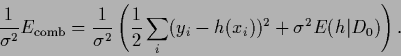
The final approximative result for the predictive density
(27)
is very simple and intuitive
.
Higher order contributions can be calculated by using Wick's theorem
[45,30,172,249,109,163,132].)
The final approximative result for the predictive density
(27)
is very simple and intuitive
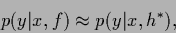 |
(71) |
with
 |
(72) |
The saddle point (or Laplace) approximation
is therefore also called Maximum A Posteriori Approximation (MAP).
Notice that the same  also maximizes
the integrand of the evidence of the data
also maximizes
the integrand of the evidence of the data 
 |
(73) |
This is due to the assumption that
 is slowly varying at the stationary point
and has not to be included in the saddle point approximation
for the predictive density.
For (functional) differentiable
is slowly varying at the stationary point
and has not to be included in the saddle point approximation
for the predictive density.
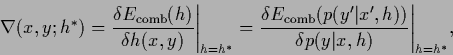
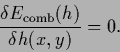
For (functional) differentiable  Eq. (72) yields the stationarity equation,
 |
(74) |
The functional including
training and prior data (regularization, stabilizer) terms
is also known as (regularized) error functional for .
In practice a saddle point approximation may be expected
useful if the posterior is peaked enough around a single maximum,
or more general, if the posterior is well approximated
by a Gaussian centered at the maximum.
For asymptotical results one would have to require
 |
(75) |
to become  -independent
for
-independent
for
 with some being the same
for the prior and data term.
(See [40,242]).
If for example
with some being the same
for the prior and data term.
(See [40,242]).
If for example
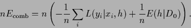
 converges for large number
  of training data
the low temperature limit
of training data
the low temperature limit
 can be interpreted
as large data limit
can be interpreted
as large data limit
 ,
,
 |
(76) |
Notice, however, the factor  in front of the prior energy.
For Gaussian temperature
corresponds to variance
in front of the prior energy.
For Gaussian temperature
corresponds to variance 
 |
(77) |
For Gaussian prior this would require simultaneous scaling
of data and prior variance.
We should also remark that for continuous ,
the stationary solution
needs not to be a typical representative of the process
 .
A common example is a
Gaussian stochastic process
with prior energy
.
A common example is a
Gaussian stochastic process
with prior energy  related to some smoothness measure of
expressed by derivatives of .
Then, even if the stationary is smooth,
this needs not to be the case for a typical
sampled according to .
For Brownian motion, for instance,
a typical sample path is not even differentiable (but continuous)
while the stationary path is smooth.
Thus, for continuous variables
only expressions like
related to some smoothness measure of
expressed by derivatives of .
Then, even if the stationary is smooth,
this needs not to be the case for a typical
sampled according to .
For Brownian motion, for instance,
a typical sample path is not even differentiable (but continuous)
while the stationary path is smooth.
Thus, for continuous variables
only expressions like
 can be given an exact meaning as a Gaussian measure,
defined by a given covariance with existing normalization factor,
but not the expressions
can be given an exact meaning as a Gaussian measure,
defined by a given covariance with existing normalization factor,
but not the expressions  and
and  alone
[51,62,228,110,83,144].
alone
[51,62,228,110,83,144].
Interestingly, the stationary
yielding maximal posterior
is not only useful to obtain an approximation
for the predictive density
 but is also the optimal solution
  for a Bayesian decision problem with log-loss
and
for a Bayesian decision problem with log-loss
and  .
.
Indeed, for a Bayesian decision problem with log-loss (46)
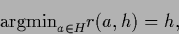 |
(78) |
and analogously,
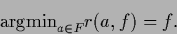 |
(79) |
This is proved as follows:
Jensen's inequality states that
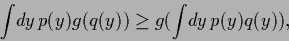 |
(80) |
for any convex function  and probability
  with
with
 .
Thus, because the logarithm is concave
.
Thus, because the logarithm is concave
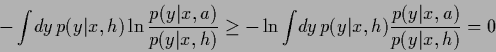 |
(81) |
 |
(82) |
with equality for  .
Hence
.
Hence
with equality for .
For  replace
  by
by  .
This proves Eqs. (78) and (79).
.
This proves Eqs. (78) and (79).
Next: Normalization, non-negativity, and specific
Up: Bayesian framework
Previous: General loss functions and
Contents
Joerg_Lemm
2001-01-21