Next: Empirical risk minimization
Up: Bayesian framework
Previous: Maximum A Posteriori Approximation
Contents
Density estimation problems are characterized by
their normalization and non-negativity condition for
 .
Thus, the prior density
.
Thus, the prior density  can only be non-zero for such
  for which is positive and normalized over
  for all
  .
(Similarly, when solving for a distribution function,
i.e., the integral of a density,
the non-negativity constraint is replaced by monotonicity and
the normalization constraint
by requiring the distribution function to be 1
on the right boundary.)
While the non-negativity constraint
is local with respect to
and , the normalization constraint
is nonlocal with respect to .
Thus, implementing a normalization constraint
leads to nonlocal and in general non-Gaussian priors.
.
(Similarly, when solving for a distribution function,
i.e., the integral of a density,
the non-negativity constraint is replaced by monotonicity and
the normalization constraint
by requiring the distribution function to be 1
on the right boundary.)
While the non-negativity constraint
is local with respect to
and , the normalization constraint
is nonlocal with respect to .
Thus, implementing a normalization constraint
leads to nonlocal and in general non-Gaussian priors.
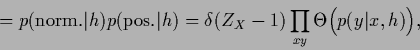
For classification problems, having discrete values (classes),
the normalization constraint
requires simply to sum over the different classes
and a Gaussian prior structure with respect to the -dependency
is not altered [236].
For general density estimation problems, however, i.e.,
for continuous , the loss of the Gaussian
structure with respect to is more severe,
because non-Gaussian functional integrals can in general not
be performed analytically.
On the other hand,
solving the learning problem
numerically by discretizing the and variables,
the normalization term is
typically not a severe complication.
To be specific,
consider a Maximum A Posteriori Approximation,
minimizing
 |
(87) |
where the likelihood free energy
 is included,
but not the prior free energy
is included,
but not the prior free energy  which, being -independent,
is irrelevant for minimization with respect to
which, being -independent,
is irrelevant for minimization with respect to  .
The prior energy
.
The prior energy
 has to implement
the non-negativity and normalization conditions
has to implement
the non-negativity and normalization conditions
It is useful to isolate the normalization condition
and non-negativity constraint defining
the class of density estimation problems
from the rest of the problem specific priors.
Introducing the specific prior information  so that
 =
=
 ,
we have
,
we have
 |
(90) |
with deterministic, -independent
 |
(91) |
 |
(92) |
and step function  .
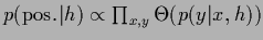
( The density
.
( The density
 is normalized over all possible normalizations of
  ,
i.e., over all possible values of
,
i.e., over all possible values of  , and
, and
 over all possible sign combinations.)
The -independent denominator
over all possible sign combinations.)
The -independent denominator
 can be skipped for error minimization with respect to .
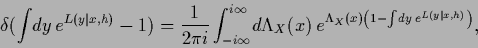
We define the specific prior as
can be skipped for error minimization with respect to .
We define the specific prior as
 |
(93) |
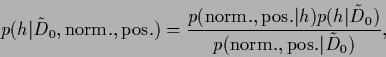
In Eq. (93)
the specific prior appears
as posterior of a -generating process
determined by the parameters .
We will call therefore Eq. (93)
the posterior form of the specific prior.
Alternatively,
a specific prior can also be in likelihood form
 |
(94) |
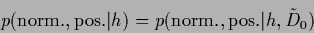
As the likelihood
 is conditioned on this means
that the normalization
is conditioned on this means
that the normalization
 =
=
 remains in general -dependent and must be included
when minimizing with respect to .
However,
Gaussian specific priors with -independent covariances
have the special property
that according to Eq. (70)
likelihood and posterior interpretation coincide.
Indeed,
representing Gaussian
specific prior data by a mean function
remains in general -dependent and must be included
when minimizing with respect to .
However,
Gaussian specific priors with -independent covariances
have the special property
that according to Eq. (70)
likelihood and posterior interpretation coincide.
Indeed,
representing Gaussian
specific prior data by a mean function
 and covariance
 (analogous to standard training data in the case of Gaussian regression,
see also Section 3.5)
one finds
due to the fact that the normalization
of a Gaussian is independent of the mean
(for uniform (meta) prior
(analogous to standard training data in the case of Gaussian regression,
see also Section 3.5)
one finds
due to the fact that the normalization
of a Gaussian is independent of the mean
(for uniform (meta) prior  )
)
Thus, for Gaussian
 with -independent
normalization the specific prior energy in likelihood form
becomes analogous to Eq. (93)
with -independent
normalization the specific prior energy in likelihood form
becomes analogous to Eq. (93)
 |
(97) |
and specific prior energies can be interpreted
both ways.
Similarly,
the complete likelihood factorizes
 |
(98) |
According to Eq. (92)
non-negativity and normalization conditions are implemented by step
and  -functions.
The non-negativity constraint is only active
when there are locations with =
-functions.
The non-negativity constraint is only active
when there are locations with =  .
In all other cases the gradient has no component
pointing into forbidden regions.
Due to the combined effect
of data, where has to be larger than zero by definition,
and smoothness terms
the non-negativity condition for
is usually (but not always) fulfilled.
Hence, if strict positivity is checked for the final solution,
then it is not necessary to include
extra non-negativity terms in the error (see Section 3.2.1).
For the sake of simplicity we will therefore not include non-negativity
terms explicitly in the following.
In case a non-negativity constraint has to be included
this can be done using Lagrange multipliers, or
alternatively, by writing the step functions in
.
In all other cases the gradient has no component
pointing into forbidden regions.
Due to the combined effect
of data, where has to be larger than zero by definition,
and smoothness terms
the non-negativity condition for
is usually (but not always) fulfilled.
Hence, if strict positivity is checked for the final solution,
then it is not necessary to include
extra non-negativity terms in the error (see Section 3.2.1).
For the sake of simplicity we will therefore not include non-negativity
terms explicitly in the following.
In case a non-negativity constraint has to be included
this can be done using Lagrange multipliers, or
alternatively, by writing the step functions in
 |
(99) |
and solving the  -integral in saddle point approximation
(See for example [63,64,65]).
-integral in saddle point approximation
(See for example [63,64,65]).
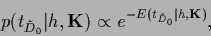
Including the normalization condition
in the prior  in form of a -functional
results in a posterior probability
in form of a -functional
results in a posterior probability
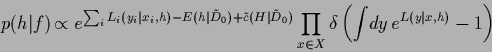 |
(100) |
with constant
 =
=
 related to the normalization
of the specific prior
related to the normalization
of the specific prior
 .
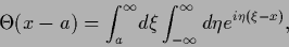
Writing the -functional
in its Fourier representation
.
Writing the -functional
in its Fourier representation
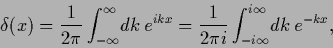 |
(101) |
i.e.,
 |
(102) |
and performing a saddle point approximation
with respect to
 (which is exact in this case)
yields
(which is exact in this case)
yields
 |
(103) |
This is equivalent to the Lagrange multiplier approach.
Here the stationary
is the Lagrange multiplier vector (or function)
to be determined by the normalization conditions
for
 .
Besides the Lagrange multiplier terms
it is numerically sometimes useful to add additional
terms to the log-posterior which vanish for normalized .
.
Besides the Lagrange multiplier terms
it is numerically sometimes useful to add additional
terms to the log-posterior which vanish for normalized .
Next: Empirical risk minimization
Up: Bayesian framework
Previous: Maximum A Posteriori Approximation
Contents
Joerg_Lemm
2001-01-21