Next: Predictive density
Up: Basic model and notations
Previous: Energies, free energies, and
Contents
Bayesian approaches require the calculation of posterior densities.
Model states  are commonly specified
by giving the data generating probabilities or likelihoods
are commonly specified
by giving the data generating probabilities or likelihoods  .
Posteriors are linked to likelihoods
by Bayes' theorem
.
Posteriors are linked to likelihoods
by Bayes' theorem
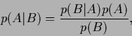 |
(14) |
which follows at once from
the definition of conditional probabilities, i.e.,
 =
=  =
=  .
Thus, one finds
.
Thus, one finds
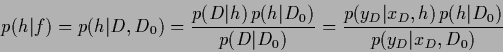 |
(15) |
 |
(16) |
using
 =
=
 for the training data likelihood of and
 =
=  .
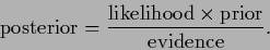
The terms of Eq. (15)
are in a Bayesian context often referred to as
.
The terms of Eq. (15)
are in a Bayesian context often referred to as
 |
(17) |
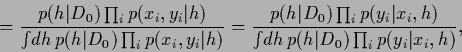
Eqs.(16) show that
the posterior can be expressed equivalently
by the joint likelihoods
 or conditional
likelihoods
or conditional
likelihoods
 .
When working with joint likelihoods, a distinction between
.
When working with joint likelihoods, a distinction between
 and
and  variables is not necessary.
In that case can be included in and skipped from the notation.
If, however,
variables is not necessary.
In that case can be included in and skipped from the notation.
If, however,  is already known or is not of interest
working with conditional likelihoods is preferable.
Eqs.(15,16) can be interpreted
as updating (or learning) formula
used to obtain a new posterior
from a given prior probability
if new data
is already known or is not of interest
working with conditional likelihoods is preferable.
Eqs.(15,16) can be interpreted
as updating (or learning) formula
used to obtain a new posterior
from a given prior probability
if new data  arrive.
In terms of energies Eq. (16) reads,
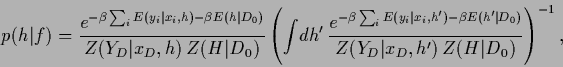 |
(18) |
where the same temperature  has been chosen for both energies
and the normalization constants are
has been chosen for both energies
and the normalization constants are
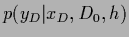
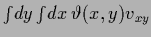
The predictive density we are interested in can be written as
the ratio of two correlation functions under  ,
,
where
 denotes the expectation
under the prior density
=
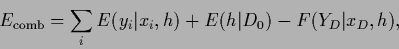
and the combined likelihood and prior energy
denotes the expectation
under the prior density
=
and the combined likelihood and prior energy  collects the -dependent energy and free energy terms
 |
(24) |
with
 |
(25) |
Going from Eq. (22)
to Eq. (23)
the normalization factor
 appearing in numerator and denominator
has been canceled.
appearing in numerator and denominator
has been canceled.
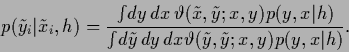
We remark that for continuous and/or
the likelihood energy term
 describes an ideal,
non-realistic measurement because
realistic measurements cannot be arbitrarily sharp.
Considering the function
describes an ideal,
non-realistic measurement because
realistic measurements cannot be arbitrarily sharp.
Considering the function
 as element of a Hilbert space
its values may be written as scalar product
=
as element of a Hilbert space
its values may be written as scalar product
=
 with a function
  being also an element in that Hilbert space.
For continuous and/or this notation is only formal
as becomes unnormalizable.
In practice a measurement of
corresponds to a normalizable
being also an element in that Hilbert space.
For continuous and/or this notation is only formal
as becomes unnormalizable.
In practice a measurement of
corresponds to a normalizable
 =
=
 where the kernel
 has to ensure normalizability.
(Choosing normalizable
as coordinates
the Hilbert space of
is also called a reproducing kernel Hilbert space
[183,112,113,228,144].)
The data terms then become
has to ensure normalizability.
(Choosing normalizable
as coordinates
the Hilbert space of
is also called a reproducing kernel Hilbert space
[183,112,113,228,144].)
The data terms then become
 |
(26) |
The notation
is understood as limit
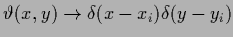 and means in practice
that
is very sharply centered.
We will assume that the discretization,
finally necessary to do numerical calculations,
will implement such an averaging.
and means in practice
that
is very sharply centered.
We will assume that the discretization,
finally necessary to do numerical calculations,
will implement such an averaging.
Next: Predictive density
Up: Basic model and notations
Previous: Energies, free energies, and
Contents
Joerg_Lemm
2001-01-21