


Next: Numerical examples
Up: Initial configurations and kernel
Previous: Kernels for
Contents
For  the truncated equation
 |
(696) |
is still nonlinear in  .
If we solve this equation approximately by a one-step iteration
.
If we solve this equation approximately by a one-step iteration
 =
=
 starting from a uniform initial
  and normalizing afterwards
this corresponds for a single
and normalizing afterwards
this corresponds for a single  -value
to the
classical kernel methods commonly used in density estimation.
As normalized density results
-value
to the
classical kernel methods commonly used in density estimation.
As normalized density results
 |
(697) |
i.e.,
 |
(698) |
with (data dependent) normalized kernel
 =
=
 and
and
 the diagonal matrix with diagonal elements
 .
Again
.
Again
 or similar invertible choices can be used
to obtain a starting guess for .
The form of the Hessian (182) suggests in particular to include
a mass term on the data.
or similar invertible choices can be used
to obtain a starting guess for .
The form of the Hessian (182) suggests in particular to include
a mass term on the data.
It would be interesting to interpret Eq. (698)
as stationarity equation of a functional  containing the usual data term
 .
Therefore, to obtain the derivative
.
Therefore, to obtain the derivative  of this data term we multiply for existing
 Eq. (698) by
 ,
where
,
where  at data points,
to obtain
at data points,
to obtain
 |
(699) |
with data dependent
 |
(700) |
Thus, Eq. (698)
is the stationarity equation of the functional
 |
(701) |
To study the dependence on the number  of training data
for a given
of training data
for a given  consider a normalized kernel with
 ,
,
 .
For such a kernel the denominator of
is equal to
.
For such a kernel the denominator of
is equal to  so we have
 |
(702) |
Assuming that for large the
empirical average
 in the denominator of
 becomes independent,
e.g., converging to the true average
becomes independent,
e.g., converging to the true average
 ,
the regularizing term in functional (701)
becomes proportional to
,
the regularizing term in functional (701)
becomes proportional to
 |
(703) |
According to Eq. (76)
this would allow to relate a
saddle point approximation to a large -limit.
Again, a similar possibility
is to start with the
empirical density
 defined in Eq. (238).
Analogously to Eq. (686),
the empirical density can for example also be smoothed
and correctly normalized again, so that
defined in Eq. (238).
Analogously to Eq. (686),
the empirical density can for example also be smoothed
and correctly normalized again, so that
 |
(704) |
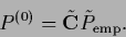
with
 defined in Eq. (698).
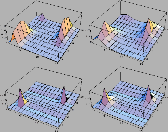
Fig. 13
compares the initialization according to
Eq. (697),
where the smoothing operator  acts on
  ,
with an initialization according to
Eq. (704),
where the smoothing operator
acts on the correctly normalized
.
,
with an initialization according to
Eq. (704),
where the smoothing operator
acts on the correctly normalized
.
Figure 13:
Comparison of initial guesses  for a case with two data points located
at
for a case with two data points located
at  and
and  within the intervals
 ![$y\in [1,15]$](img100.png) and
and ![$x\in [1,10]$](img101.png) with periodic boundary conditions.
First row: =
with periodic boundary conditions.
First row: =
 .
(The smoothing operator
acts on the unnormalized .
The following conditional normalization changes the
shape more drastically than in the example shown in the second row.)
Second row: =
.
(The smoothing operator
acts on the unnormalized .
The following conditional normalization changes the
shape more drastically than in the example shown in the second row.)
Second row: =
 .
(The smoothing operator
acts on the already conditionally normalized
.
(The smoothing operator
acts on the already conditionally normalized
 .)
The kernel
.)
The kernel
 is given by Eq. (698)
with
is given by Eq. (698)
with  =
=
 ,
,
 =
=  ,
and a
,
and a  of the form of Eq. (705)
with
of the form of Eq. (705)
with
 =
=  =
=  = 0,
and
= 0,
and
 =
=  (figures on the l.h.s.)
or
= (figures on the r.h.s.),
respectively.
(figures on the l.h.s.)
or
= (figures on the r.h.s.),
respectively.
 |
Next: Numerical examples
Up: Initial configurations and kernel
Previous: Kernels for
Contents
Joerg_Lemm
2001-01-21