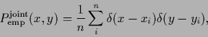
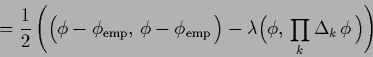
Interpreting an energy or error functional ![]() probabilistically,
i.e., assuming
probabilistically,
i.e., assuming ![]() to be the logarithm of a posterior probability under study,
the form of the training data term has to be
to be the logarithm of a posterior probability under study,
the form of the training data term has to be
![]() .
Technically, however, it would be easier to replace
that data term by one which is quadratic in the function
.
Technically, however, it would be easier to replace
that data term by one which is quadratic in the function
![]() of interest.
of interest.
Indeed, we have mentioned in Section 2.5
that such functionals can be justified
within the framework of empirical risk minimization.
From that Frequentist point of view an error functional ![]() ,
is not derived from a log-posterior,
but represents an empirical risk
,
is not derived from a log-posterior,
but represents an empirical risk
![]() ,
approximating an
expected risk
,
approximating an
expected risk ![]() for action
for action ![]() =
= ![]() .
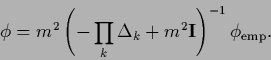
This is possible under the assumption that
training data are sampled according to the true
.
This is possible under the assumption that
training data are sampled according to the true ![]() .
In that interpretation
one is therefore not restricted to
a log-loss for training data
but may as well choose for training data a quadratic loss like
.
In that interpretation
one is therefore not restricted to
a log-loss for training data
but may as well choose for training data a quadratic loss like
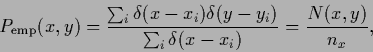
Approximating a joint probability ![]() the reference density
the reference density ![]() would have to be the joint empirical density
would have to be the joint empirical density
Hence, approximating conditional empirical densities
either non-data ![]() -values must be excluded
from the integration in (234)
by using an operator
-values must be excluded
from the integration in (234)
by using an operator ![]() containing the projector
containing the projector
![]() ,
or
,
or ![]() must be defined also for such non-data
must be defined also for such non-data ![]() -values.
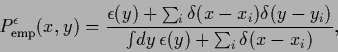
For existing
-values.
For existing
![]() =
= ![]() =
=
![]() ,
a possible extension
,
a possible extension
![]() of
of ![]() would be to assume a uniform density for non-data
would be to assume a uniform density for non-data ![]() values,
yielding
values,
yielding
Instead of a quadratic term in ![]() ,
one might consider a quadratic term in the log-probability
,
one might consider a quadratic term in the log-probability ![]() .
The log-probability, however,
is minus infinity at all non-data points
.
The log-probability, however,
is minus infinity at all non-data points
![]() .
To work with a finite expression, one can choose
small
.
To work with a finite expression, one can choose
small ![]() and approximate
and approximate ![]() by
by
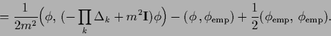
A quadratic data term in ![]() results in an error functional
results in an error functional
Positive (semi-)definite operators ![]() have a square root and can be written
in the form
have a square root and can be written
in the form
![]() .
One possibility,
skipping for the sake of simplicity
.
One possibility,
skipping for the sake of simplicity ![]() in the following,
is to choose
as square root
in the following,
is to choose
as square root ![]() the integration operator, i.e.,
the integration operator, i.e.,
![]() =
=
![]() and
and
![]() =
=
![]() .
Thus,
.
Thus,
![]() transforms the density function
transforms the density function ![]() in the distribution function
in the distribution function ![]() ,
and we have
,
and we have
![]() .
Here the inverse
.
Here the inverse ![]() is the differentiation operator
is the differentiation operator
![]() (with appropriate boundary conditions)
and
(with appropriate boundary conditions)
and
 =
=
![]() is the product of one-dimensional Laplacians
is the product of one-dimensional Laplacians
![]() .
Adding for example a regularizing term
.
Adding for example a regularizing term
![]() as in (165)
gives
as in (165)
gives