Next: Gaussian relaxation
Up: Learning matrices
Previous: Linearization and Newton algorithm
Contents
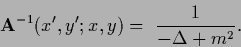
Massive relaxation
We now consider methods to construct a
positive definite or at least invertible learning matrix.
For example, far from a minimum the Hessian  may not be positive definite
and like a differential operator
may not be positive definite
and like a differential operator  with zero modes, not even invertible.
Massive relaxation
can transform a non-invertible or not positive definite operator
with zero modes, not even invertible.
Massive relaxation
can transform a non-invertible or not positive definite operator  ,
e.g.
,
e.g.
 or
or
 ,
into an invertible or positive definite operators:
,
into an invertible or positive definite operators:
A generalization would be to allow  .
This is, for example, used
in some realizations of Newton`s method for minimization
in regions where is not positive definite
and a diagonal operator is added to
.
This is, for example, used
in some realizations of Newton`s method for minimization
in regions where is not positive definite
and a diagonal operator is added to  ,
using for example a modified Cholesky factorization
[19].
The mass term removes the zero modes of
if
,
using for example a modified Cholesky factorization
[19].
The mass term removes the zero modes of
if  is not in the spectrum of
and makes it positive definite if
is not in the spectrum of
and makes it positive definite if  is larger than the smallest eigenvalue of .
Matrix elements
is larger than the smallest eigenvalue of .
Matrix elements
 of the resolvent
 ,
,
 representing in this case a complex variable,
have poles at discrete eigenvalues of
and a cut at the continuous spectrum
as long as
representing in this case a complex variable,
have poles at discrete eigenvalues of
and a cut at the continuous spectrum
as long as  has a non-zero overlap with
the corresponding eigenfunctions.
Instead of multiples of the identity,
also other operators may be added to remove zero modes.
The Hessian
has a non-zero overlap with
the corresponding eigenfunctions.
Instead of multiples of the identity,
also other operators may be added to remove zero modes.
The Hessian  in (156), for example,
adds a
in (156), for example,
adds a  -dependent mass-like, but not necessarily positive definite
term to .
Similarly, for example
-dependent mass-like, but not necessarily positive definite
term to .
Similarly, for example  in (182) has
 -dependent mass
 restricted to data points.
While full relaxation is the massless limit
 of massive
relaxation, a gradient algorithm with
of massive
relaxation, a gradient algorithm with  can be obtained
as infinite mass limit
can be obtained
as infinite mass limit
 with
with
 and
and
 .
.
Constant functions are typical zero modes, i.e.,
eigenfunctions with zero eigenvalue,
for differential operators
with periodic boundary conditions.
For instance for a common smoothness term
 (kinetic energy operator)
as regularizing operator
the inverse of
(kinetic energy operator)
as regularizing operator
the inverse of
 has the form
 |
(639) |
 |
(640) |
with  ,
,  = dim(
 ),
),  = dim(
 ).
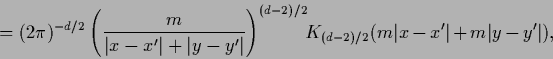
This Green`s function or matrix element of the resolvent kernel
for is analogous to the (Euclidean) propagator
of a free scalar field with mass
).
This Green`s function or matrix element of the resolvent kernel
for is analogous to the (Euclidean) propagator
of a free scalar field with mass  ,
which is its two-point correlation function
or matrix element of the covariance operator.
According to
,
which is its two-point correlation function
or matrix element of the covariance operator.
According to
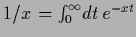 the denominator can be brought into the exponent
by introducing an additional integral.
Performing the resulting Gaussian integration over
the denominator can be brought into the exponent
by introducing an additional integral.
Performing the resulting Gaussian integration over  the inverse can be expressed as
 |
(641) |
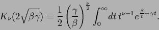
in terms of the
modified Bessel functions  which
have the following integral representation
which
have the following integral representation
 |
(642) |
Alternatively, the same result can be obtained
by switching to  -dimensional spherical coordinates,
expanding the exponential in ultra-spheric harmonic functions
and performing the integration over the angle-variables
[117].
For the example
-dimensional spherical coordinates,
expanding the exponential in ultra-spheric harmonic functions
and performing the integration over the angle-variables
[117].
For the example  this corresponds to Parzen´s kernel
used in density estimation
or for
this corresponds to Parzen´s kernel
used in density estimation
or for 
 |
(643) |
The Green's function for periodic, Neumann, or Dirichlet boundary conditions
can be expressed by sums over
 [77].
[77].
The lattice version
of the Laplacian with lattice spacing  reads
reads
![\begin{displaymath}
\hat \Delta f(n) =
\frac{1}{a^2} \sum_j^d
[ f(n-a_j)-2 f(n) + f(n+a_j) ],
\end{displaymath}](img2127.png) |
(644) |
writing  for a vector in direction
  and length .
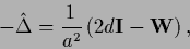
Including a mass term
we get as lattice approximation for
and length .
Including a mass term
we get as lattice approximation for 
 |
(645) |
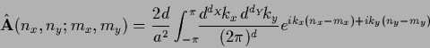
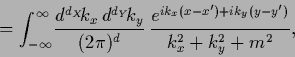
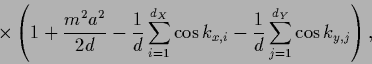
Inserting the Fourier representation (101)
of  gives
gives
 |
(646) |
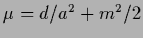
with  =
=  ,
,  =
=
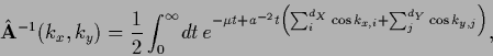
 and inverse
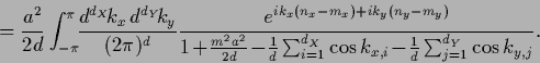 |
(647) |
(For  and
and  the integrand diverges
for
the integrand diverges
for
 (infrared divergence).
Subtracting formally the also infinite
(infrared divergence).
Subtracting formally the also infinite
 results in finite difference.
For example in one finds
results in finite difference.
For example in one finds
 =
=
 [103].
Using
one obtains [195]
[103].
Using
one obtains [195]
 |
(648) |
with
 .
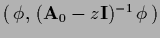
This allows to express the inverse
.
This allows to express the inverse
 in terms of the modified Bessel functions
  which have for integer argument
  the integral representation
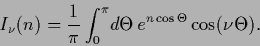 |
(649) |
One finds
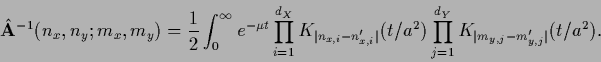 |
(650) |
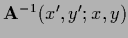
It might be interesting to remark that the matrix elements of the
inverse learning matrix or free massive propagator
on the lattice
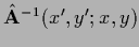 can be given an interpretation
in terms of (random) walks connecting the two points
can be given an interpretation
in terms of (random) walks connecting the two points
 and
[56,195].
For that purpose
the lattice Laplacian is splitted into a diagonal and a nearest neighbor part
and
[56,195].
For that purpose
the lattice Laplacian is splitted into a diagonal and a nearest neighbor part
 |
(651) |
where the nearest neighbor matrix
 has matrix elements equal one for nearest neighbors
and equal to zero otherwise.
Thus,
has matrix elements equal one for nearest neighbors
and equal to zero otherwise.
Thus,
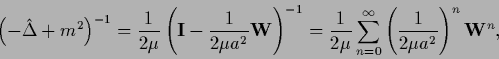 |
(652) |
can be written as geometric series.
The matrix elements
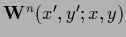 give the number of walks
![$w[(x^\prime,y^\prime)\rightarrow (x,y)]$](img2156.png) of length
of length  = connecting
the two points
and .
Thus, one can write
= connecting
the two points
and .
Thus, one can write
![\begin{displaymath}
\left( - \hat \Delta + m^2\right)^{-1}(x^\prime,y^\prime;x,y...
...rrow (x,y)]}
\left(\frac{1}{2 \mu a^2}\right)^{\vert w\vert} .
\end{displaymath}](img2158.png) |
(653) |
Next: Gaussian relaxation
Up: Learning matrices
Previous: Linearization and Newton algorithm
Contents
Joerg_Lemm
2001-01-21