Next: Gaussian prior factor for
Up: Gaussian prior factor for
Previous: Normalization by parameterization: Error
Contents
The Hessians  ,
, 
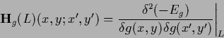
The Hessian of  is defined as the matrix or operator of second derivatives
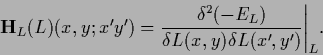 |
(154) |
For functional (109)
and fixed  we find the Hessian by taking the derivative
of the gradient in (127) with respect to
we find the Hessian by taking the derivative
of the gradient in (127) with respect to  again.
This gives
again.
This gives
 |
(155) |
or
 |
(156) |
The addition of the diagonal matrix
 =
=
 can result in a negative definite
 even if
  has zero modes,
like for a differential operator
with periodic boundary conditions.
Note, however, that
is diagonal and therefore symmetric,
but not necessarily positive definite, because
has zero modes,
like for a differential operator
with periodic boundary conditions.
Note, however, that
is diagonal and therefore symmetric,
but not necessarily positive definite, because  can be negative
for some
can be negative
for some  . Depending on the sign of
the normalization condition
. Depending on the sign of
the normalization condition  for that can be replaced
by the inequality
for that can be replaced
by the inequality  or
or  .
Including the -dependence of and with
.
Including the -dependence of and with
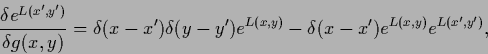 |
(157) |
i.e.,
 |
(158) |
or
 |
(159) |
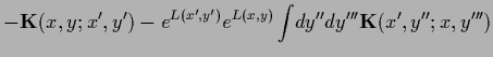
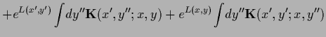
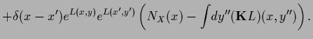
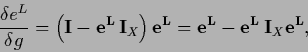
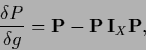
we find, written in terms of ,
The last term, diagonal in  , has dyadic structure in
  ,
and therefore for fixed at most one non-zero eigenvalue.
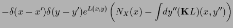
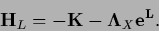
In matrix notation the Hessian becomes
,
and therefore for fixed at most one non-zero eigenvalue.
In matrix notation the Hessian becomes
the second line written in terms of the probability matrix.
The expression is symmetric under
 ,
,
 ,
as it must be for a Hessian and as can be verified using the symmetry of
,
as it must be for a Hessian and as can be verified using the symmetry of
 and the fact that
 and
and  commute, i.e.,
![$[{\bf\Lambda}_X , {\bf I}_X] = 0$](img650.png) .
Because functional
.
Because functional  is invariant under a shift transformation,
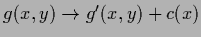 , the Hessian has
a space of zero modes with the dimension of .
Indeed,
any
, the Hessian has
a space of zero modes with the dimension of .
Indeed,
any  -independent function
(which can have finite
-independent function
(which can have finite
 -norm only in finite -spaces)
is a left eigenvector of
-norm only in finite -spaces)
is a left eigenvector of
 with eigenvalue zero.
Thus, where necessary,
the pseudo inverse of have to be used instead of the inverse.
Alternatively, additional constraints on
with eigenvalue zero.
Thus, where necessary,
the pseudo inverse of have to be used instead of the inverse.
Alternatively, additional constraints on  can be added
which remove zero modes,
like for example boundary conditions.
can be added
which remove zero modes,
like for example boundary conditions.
Next: Gaussian prior factor for
Up: Gaussian prior factor for
Previous: Normalization by parameterization: Error
Contents
Joerg_Lemm
2001-01-21