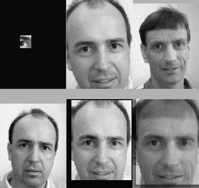
As numerical example we study a
two component mixture model for image completion.
Assume we expect an only partially known image
(corresponding to pixel-wise training data
drawn with Gaussian noise from the original image)
to be similar to one of the two template images shown
in Fig.4.
Next, we include hyperparameters parameterising deformations of templates.
In particular, we have chosen
translations (![]() ,
, ![]() )
a scaling factor
)
a scaling factor ![]() ,
and a rotation angle (around template center)
,
and a rotation angle (around template center)
![]() .
.
Interestingly,
it turned out that due to the large number of data
(
![]() 1000) it was easier
to solve Eq.(21) for the full discretized image
than to invert (32) in the space of training data.
A prior operator
1000) it was easier
to solve Eq.(21) for the full discretized image
than to invert (32) in the space of training data.
A prior operator ![]() has been implemented
as a
has been implemented
as a ![]() negative Laplacian filter.
(Notice that using a Laplacian kernel, or another smoothness measure,
instead of a straight template matching
using simply the squared error between image and template,
leads to a smooth interpolation between data and templates.)
Completed images
negative Laplacian filter.
(Notice that using a Laplacian kernel, or another smoothness measure,
instead of a straight template matching
using simply the squared error between image and template,
leads to a smooth interpolation between data and templates.)
Completed images ![]() for different
for different ![]() have been found by iterating according to
have been found by iterating according to
![\begin{displaymath}
h^{k+1} = h^k + \eta {\bf A}^{-1}
\Big[
{\bf K}_T (t_T-h^k)
+ {\bf K}_0 \Big(\sum_j a_j^k t_j -h^k\Big)
\Big]
,
\end{displaymath}](img221.gif) |
(47) |
Being a mixture model with ![]() the situation is that of Fig.3.
Typical solutions for large and small
the situation is that of Fig.3.
Typical solutions for large and small ![]() are shown in Fig.4.
are shown in Fig.4.
 |