Next: Learning matrices
Up: Iteration procedures: Learning
Previous: Iteration procedures: Learning
Contents
Due to the presence of the logarithmic
data term  and the normalization constraint in density estimation problems
the stationary equations are in general nonlinear,
even for Gaussian specific priors.
An exception are Gaussian regression problems
discussed in Section 3.7
for which becomes quadratic
and the normalization constraint can be skipped.
However, the nonlinearities
arising from the data term
are restricted to a finite number of
training data points
and for Gaussian specific priors one may expect them,
like those arising from the normalization constraint,
to be numerically not very harmful.
Clearly, severe nonlinearities can appear
for general non-Gaussian specific priors
or general nonlinear parameterizations
and the normalization constraint in density estimation problems
the stationary equations are in general nonlinear,
even for Gaussian specific priors.
An exception are Gaussian regression problems
discussed in Section 3.7
for which becomes quadratic
and the normalization constraint can be skipped.
However, the nonlinearities
arising from the data term
are restricted to a finite number of
training data points
and for Gaussian specific priors one may expect them,
like those arising from the normalization constraint,
to be numerically not very harmful.
Clearly, severe nonlinearities can appear
for general non-Gaussian specific priors
or general nonlinear parameterizations  .
.
As nonlinear equations the stationarity conditions
have in general to be solved by iteration.
In the context of empirical learning iteration procedures
to minimize an error functional represent possible learning algorithms.
In the previous sections we have encountered
stationarity equations
 |
(607) |
for error functionals  , e.g.,
  =
=  or =
or =  ,
written in a form
,
written in a form
 |
(608) |
with -dependent  (and possibly
  ).
For the stationarity Eqs. (143), (172),
and (193)
the operator
).
For the stationarity Eqs. (143), (172),
and (193)
the operator  is a
-independent inverse covariance
of a Gaussian specific prior.
It has already been mentioned that for existing
(and not too ill-conditioned)
is a
-independent inverse covariance
of a Gaussian specific prior.
It has already been mentioned that for existing
(and not too ill-conditioned)
 (representing the covariance of the prior process)
Eq. (608)
suggests an iteration scheme
(representing the covariance of the prior process)
Eq. (608)
suggests an iteration scheme
 |
(609) |
for discretized starting from some initial guess  .
In general, like for the non-Gaussian specific priors discussed in
Section 6,
can be -dependent.
Eq. (368) shows that general nonlinear parameterizations
lead to nonlinear operators .
.
In general, like for the non-Gaussian specific priors discussed in
Section 6,
can be -dependent.
Eq. (368) shows that general nonlinear parameterizations
lead to nonlinear operators .
Clearly,
if allowing -dependent ,
the form (608) is no restriction of generality.
One always can choose an arbitrary invertible (and not too ill-conditioned)
 ,
define
,
define
 |
(610) |
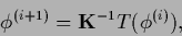
write a stationarity equation as
 |
(611) |
discretize and iterate with  .
To obtain a numerical iteration scheme
we will choose
a linear, positive definite learning matrix .
The learning matrix may depend on
and may also change during iteration.
.
To obtain a numerical iteration scheme
we will choose
a linear, positive definite learning matrix .
The learning matrix may depend on
and may also change during iteration.
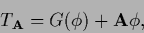
To connect a stationarity equation given in form (608)
to an arbitrary iteration scheme with
a learning matrix
we define
 |
(612) |
i.e., we split into two parts
 |
(613) |
where we introduced  for later convenience.
Then we obtain from the stationarity equation (608)
for later convenience.
Then we obtain from the stationarity equation (608)
 |
(614) |
To iterate we start by inserting an approximate solution
 to the right-hand side
and obtain a new
to the right-hand side
and obtain a new  by calculating the left hand side.
This can be written in one of the following equivalent forms
by calculating the left hand side.
This can be written in one of the following equivalent forms
where plays the role of a learning rate
or step width,
and =
 may be iteration dependent.
The update equations (615-617) can be written
may be iteration dependent.
The update equations (615-617) can be written
 |
(618) |
with
 =
=
 .
Eq. (617) does not require
the calculation of
.
Eq. (617) does not require
the calculation of  or
or  so that instead of
directly can be given
without the need to calculate its inverse.
For example operators approximating
and being easy to
calculate may be good choices for .
so that instead of
directly can be given
without the need to calculate its inverse.
For example operators approximating
and being easy to
calculate may be good choices for .
For positive definite
(and thus also positive definite inverse)
convergence can be guaranteed, at least theoretically.
Indeed,
multiplying with
 and projecting onto
an infinitesimal
and projecting onto
an infinitesimal  gives
gives
 |
(619) |
In an infinitesimal neighborhood of
where
 becomes equal to in first order
the left-hand side is for positive (semi-)definite
larger (or equal) to zero.
This shows that at least for small enough
the posterior log-probability
becomes equal to in first order
the left-hand side is for positive (semi-)definite
larger (or equal) to zero.
This shows that at least for small enough
the posterior log-probability  increases
i.e., the differential
increases
i.e., the differential  is smaller or equal to zero
and the value of the error functional decreases.
is smaller or equal to zero
and the value of the error functional decreases.
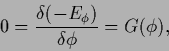
Stationarity equation
(127) for minimizing  yields for (615,616,617),
The function
 is also unknown
and is part of the variables
we want to solve for.
The normalization conditions
provide the necessary additional equations,
and the matrix can be extended
to include the iteration procedure for
is also unknown
and is part of the variables
we want to solve for.
The normalization conditions
provide the necessary additional equations,
and the matrix can be extended
to include the iteration procedure for  .
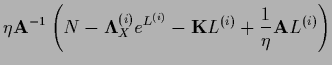
For example, we can insert the stationarity equation for
in (622) to get
.
For example, we can insert the stationarity equation for
in (622) to get
![\begin{displaymath}
L^{(i+1)} =
L^{(i)} + \eta {\bf A}^{-1}
\left[ N - e^{{\bf ...
...)}} (N_X-{\bf I}_X {{\bf K}} L)
- {{\bf K}} L^{(i)} \right] .
\end{displaymath}](img2065.png) |
(623) |
If normalizing  at each iteration this
corresponds to an iteration procedure for
at each iteration this
corresponds to an iteration procedure for
 .
.
Similarly, for the functional  we have to solve (166)
and obtain for (617),
we have to solve (166)
and obtain for (617),
Again, normalizing at each iteration this is equivalent to
solving for  ,
and the update procedure for can be varied.
,
and the update procedure for can be varied.
Next: Learning matrices
Up: Iteration procedures: Learning
Previous: Iteration procedures: Learning
Contents
Joerg_Lemm
2001-01-21