


Next: Regularization parameters
Up: Adapting prior covariances
Previous: Local masses and gauge
Contents
In this section we discuss parameterizations of the inverse covariance
of a Gaussian specific prior which leave the determinant invariant.
In that case no  -dependent normalization factors
have to be included which are usually very difficult to calculate.
We have to keep in mind, however,
that in general a large freedom for
-dependent normalization factors
have to be included which are usually very difficult to calculate.
We have to keep in mind, however,
that in general a large freedom for
 effectively diminishes the influence of the parameterized prior term.
A determinant is, for example,
invariant under general similarity transformations,
i.e.,
 =
=
 for
for
 =
=
 where
where  could be any element of the general linear group.
Similarity transformations do not change the eigenvalues,
because from
could be any element of the general linear group.
Similarity transformations do not change the eigenvalues,
because from
 =
=  follows
 =
=
 .
Thus, if
.
Thus, if  is positive definite
also
is positive definite
also
 is.
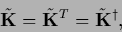
The additional constraint that
has to be real symmetric,
is.
The additional constraint that
has to be real symmetric,
 |
(469) |
requires to be real and orthogonal
 |
(470) |
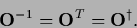
Furthermore, as an overall factor of does not change
one can restrict
to a special orthogonal group  with
with
 .
If has degenerate eigenvalues
there exist orthogonal transformations with =
.
.
If has degenerate eigenvalues
there exist orthogonal transformations with =
.
While in one dimension
only the identity remains as transformation,
the condition of an invariant determinant
becomes less restrictive in higher dimensions.
Thus, especially for large dimension  of (infinite for continuous
  )
there is a great freedom to adapt inverse covariances
without the need to calculate normalization factors,
for example to adapt the sensible directions
of a multivariate Gaussian.
)
there is a great freedom to adapt inverse covariances
without the need to calculate normalization factors,
for example to adapt the sensible directions
of a multivariate Gaussian.
A positive definite
can be diagonalized by an orthogonal matrix
with  =
=  , i.e.,
 .
Parameterizing the specific prior term becomes
.
Parameterizing the specific prior term becomes
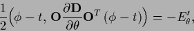
 |
(471) |
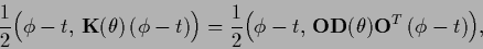
so the stationarity Eq. (459) reads
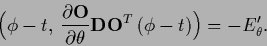 |
(472) |
Matrices from
include rotations and inversion.
For a Gaussian specific prior
with nondegenerate eigenvalues Eq. (472)
allows therefore to adapt the `sensible' directions
of the Gaussian.
There are also transformations which can change eigenvalues,
but leave eigenvectors invariant.
As example, consider a diagonal matrix  with diagonal elements (and eigenvalues)
 , i.e.,
 =
=
 .
Clearly, any permutation of the eigenvalues
.
Clearly, any permutation of the eigenvalues  leaves the determinant invariant and transforms a positive definite matrix
into a positive definite matrix.
Furthermore, one may introduce
continuous parameters
leaves the determinant invariant and transforms a positive definite matrix
into a positive definite matrix.
Furthermore, one may introduce
continuous parameters  with
with  and transform
 according to
 |
(473) |
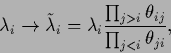
which leaves the product
 =
=
 and therefore also the determinant invariant
and transforms a positive definite matrix into a positive definite matrix.
This can be done with every pair of eigenvalues
defining a set of continuous parameters
and therefore also the determinant invariant
and transforms a positive definite matrix into a positive definite matrix.
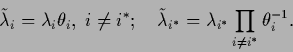
This can be done with every pair of eigenvalues
defining a set of continuous parameters
 with
( can be completed to a symmetric matrix)
leading to
with
( can be completed to a symmetric matrix)
leading to
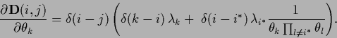
 |
(474) |
which also leaves the determinant invariant
 |
(475) |
A more general transformation with unique parameterization
by  ,
,  ,
still leaving the eigenvectors unchanged, would be
,
still leaving the eigenvectors unchanged, would be
 |
(476) |
This techniques can be applied to a general positive definite
after diagonalizing
 |
(477) |
As example consider the transformations
(474, 476)
for which the specific prior term becomes
 |
(478) |
and stationarity Eq. (459)
 |
(479) |
and for (474),
with  ,
,
 |
(480) |
or, for (476),
with  ,
,
 |
(481) |
If, for example, is a translationally invariant operator
it is diagonalized in a basis of plane waves.
Then also
is translationally invariant,
but its sensitivity to certain frequencies has changed.
The optimal sensitivity pattern is determined
by the given stationarity equations.
Next: Regularization parameters
Up: Adapting prior covariances
Previous: Local masses and gauge
Contents
Joerg_Lemm
2001-01-21