Next: Exact posterior for hyperparameters
Up: Adapting prior covariances
Previous: Invariant determinants
Contents
Next we consider the example
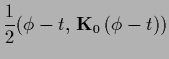
 =
=
 where
where  has been denoted
  ,
representing a regularization parameter or
an inverse temperature variable for the specific prior.
For a
,
representing a regularization parameter or
an inverse temperature variable for the specific prior.
For a  -dimensional Gaussian integral
the normalization factor becomes
-dimensional Gaussian integral
the normalization factor becomes
 =
=
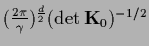 .
For positive (semi-)definite
.
For positive (semi-)definite  the dimension is
given by the rank of under a chosen discretization.
Skipping constants results in a normalization energy
the dimension is
given by the rank of under a chosen discretization.
Skipping constants results in a normalization energy
 =
=
 .
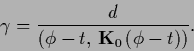
With
.
With
 |
(482) |
we obtain the stationarity equations
For compensating hyperprior
the right hand side of Eq. (484) vanishes,
giving thus no stationary point for .
Using however the condition  one sees that for positive definite
  Eq. (483)
is minimized for =
Eq. (483)
is minimized for =  corresponding to the `prior-free' case.
For example, in the case of Gaussian regression the solution
would be the data template
corresponding to the `prior-free' case.
For example, in the case of Gaussian regression the solution
would be the data template  =
=  =
=  .
This is also known as ``
.
This is also known as `` -catastrophe''.
To get a nontrivial solution for
a noncompensating hyperparameter energy
-catastrophe''.
To get a nontrivial solution for
a noncompensating hyperparameter energy  =
=  must be used
so that
must be used
so that
 is nonuniform
[16,24].
is nonuniform
[16,24].
The other limiting case is
a vanishing
 for which
Eq. (484) becomes
for which
Eq. (484) becomes
 |
(485) |
For
 one sees that
 .
Moreover, in case
.
Moreover, in case ![$P[t]$](img1673.png) represents a normalized probability,
represents a normalized probability,
 is also a solution of the first stationarity equation (483)
in the limit
.
Thus, for vanishing
the `data-free' solution
is a selfconsistent solution
of the stationarity equations (483,484).
is also a solution of the first stationarity equation (483)
in the limit
.
Thus, for vanishing
the `data-free' solution
is a selfconsistent solution
of the stationarity equations (483,484).
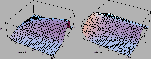
Fig.6 shows a posterior surface
for uniform and for compensating hyperprior
for a one-dimensional regression example.
The Maximum A Posteriori Approximation
corresponds to the highest point of the joint posterior
over , in that figures.
Alternatively one can treat
the -integral
by Monte-Carlo-methods [236].
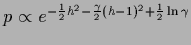
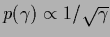
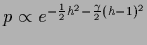
Figure 6:
Shown is the joint posterior density of and , i.e.,
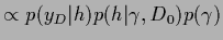 for a zero-dimensional example of Gaussian regression
with training data
for a zero-dimensional example of Gaussian regression
with training data  and prior data
  .
L.h.s:
For uniform prior
.
L.h.s:
For uniform prior
 so that the joint posterior becomes
 ,
having its maximum is at =
,
having its maximum is at =  ,
,  .
R.h.s.:
For compensating hyperprior
.
R.h.s.:
For compensating hyperprior
 so that
 having its maximum is at = ,
  .
.
 |
Finally we remark that
in the setting of empirical risk minimization,
due to the different interpretation of the error functional,
regularization parameters are usually determined by
cross-validation or similar techniques
[166,6,230,216,217,81,39,211,228,54,83].
Next: Exact posterior for hyperparameters
Up: Adapting prior covariances
Previous: Invariant determinants
Contents
Joerg_Lemm
2001-01-21