


Next: Additive models
Up: Parameterizing likelihoods: Variational methods
Previous: Linear trial spaces
Contents
Mixture models
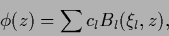
The function  can be approximated by a mixture model,
i.e., by a linear combination of components functions
can be approximated by a mixture model,
i.e., by a linear combination of components functions
 |
(390) |
with parameter vectors  and constants
  (which could also be included into the vector )
to be adapted.
The functions
(which could also be included into the vector )
to be adapted.
The functions
 are often chosen to depend on one-dimensional
combinations of the vectors and
are often chosen to depend on one-dimensional
combinations of the vectors and  .
For example they may depend on some distance
.
For example they may depend on some distance
 (`local or distance approaches')
or the projection of in -direction, i.e.,
(`local or distance approaches')
or the projection of in -direction, i.e.,
 (`projection approaches').
(For projection approaches see also Sections
4.5, 4.8 and 4.9).
(`projection approaches').
(For projection approaches see also Sections
4.5, 4.8 and 4.9).
A typical example are Radial Basis Functions (RBF)
using Gaussian
for which centers
(and possibly covariances and also number of components)
can be adjusted.
Other local methods include
 -nearest neighbors methods (NN)
and learning vector quantizations (LVQ)
and its variants.
(For a comparison see [158].)
-nearest neighbors methods (NN)
and learning vector quantizations (LVQ)
and its variants.
(For a comparison see [158].)
Joerg_Lemm
2001-01-21