Next: Parameterizing priors: Hyperparameters
Up: Parameterizing likelihoods: Variational methods
Previous: Projection pursuit
Contents
Neural networks
While in projection pursuit-like techniques
the one-dimensional `ridge' functions  are adapted optimally, neural networks use ridge functions
of a fixed sigmoidal form.
The resulting lower flexibility following from fixing the ridge function
is then compensated by iterating this parameterization.
This leads to multilayer neural networks.
are adapted optimally, neural networks use ridge functions
of a fixed sigmoidal form.
The resulting lower flexibility following from fixing the ridge function
is then compensated by iterating this parameterization.
This leads to multilayer neural networks.
Multilayer neural networks have been become a popular
tool for regression and classification problems
[205,124,159,96,167,231,24,200,10].
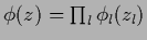
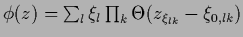
One-layer neural networks, also known as perceptrons,
correspond to the parameterization
 |
(411) |
with a sigmoidal function  ,
parameters
,
parameters  =
=  , projection
 and
and  single components of the variables
  ,
,  ,
i.e.,
,
i.e.,
 =
=  for
for  and
=
and
=  for
for
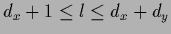 .
(For neural networks with Lorentzians instead of sigmoids
see [72].)
.
(For neural networks with Lorentzians instead of sigmoids
see [72].)
Typical choices for the sigmoid are
 =
=
 or =
or =
 .
The parameter
.
The parameter  , often called inverse temperature,
controls the sharpness of the step of the sigmoid.
In particular,
the sigmoid functions become a sharp step
in the limit
, often called inverse temperature,
controls the sharpness of the step of the sigmoid.
In particular,
the sigmoid functions become a sharp step
in the limit
 , i.e.,
at zero temperature.
In principle the sigmoidal function may depend on further parameters
which then
-- similar to projection pursuit discussed in Section 4.8 --
would also have to be included in the optimization process.
The threshold or bias
, i.e.,
at zero temperature.
In principle the sigmoidal function may depend on further parameters
which then
-- similar to projection pursuit discussed in Section 4.8 --
would also have to be included in the optimization process.
The threshold or bias  can
be treated as weight if an additional input component is included
clamped to the value
can
be treated as weight if an additional input component is included
clamped to the value  .
.
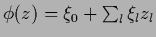
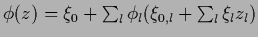
A linear combination of perceptrons
 |
(412) |
has the form of a projection pursuit approach (408)
but with fixed  =
=  .
.
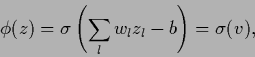
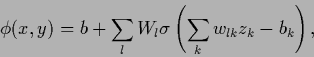
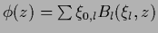
In multi-layer networks the parameterization (411) is cascaded,
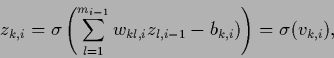 |
(413) |
with
 representing
the output of the
representing
the output of the  th node (neuron) in layer
  and
and
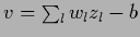
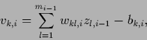 |
(414) |
being the input for that node.
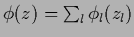
This yields, skipping the bias terms for simplicity
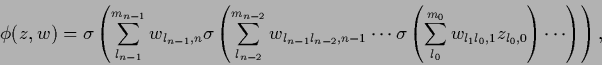 |
(415) |
beginning with an input layer
with  =
=  nodes
(plus possibly nodes to implement the bias)
nodes
(plus possibly nodes to implement the bias)
 =
and going over intermediate layers with
=
and going over intermediate layers with  nodes
nodes
 ,
,  ,
,  to a single node output layer
  =
=  .
.
Commonly neural nets are used in regression and classification
to parameterize a function =  in functionals
 |
(416) |
quadratic in  and without further regularization terms.
In that case, regularization has to be assured by
using either
1. a neural network architecture which is restrictive enough,
2. by using early stopping like training procedures
so the full flexibility of the network structure cannot
completely develop and destroy generalization,
where in both cases the optimal architecture or algorithm
can be determined
for example by cross-validation or bootstrap techniques
[166,6,230,216,217,81,39,228,54],
or
3. by averaging over ensembles of networks [170].
In all these cases regularization is implicit in the parameterization
of the network.
Alternatively, explicit regularization or prior terms
can be added to the functional.
For regression or classification
this is for example done in learning by hints
[2,3,4]
or curvature-driven smoothing with feedforward networks
[22].
and without further regularization terms.
In that case, regularization has to be assured by
using either
1. a neural network architecture which is restrictive enough,
2. by using early stopping like training procedures
so the full flexibility of the network structure cannot
completely develop and destroy generalization,
where in both cases the optimal architecture or algorithm
can be determined
for example by cross-validation or bootstrap techniques
[166,6,230,216,217,81,39,228,54],
or
3. by averaging over ensembles of networks [170].
In all these cases regularization is implicit in the parameterization
of the network.
Alternatively, explicit regularization or prior terms
can be added to the functional.
For regression or classification
this is for example done in learning by hints
[2,3,4]
or curvature-driven smoothing with feedforward networks
[22].
One may also remark
that from a Frequentist point of view the quadratic functional
is not interpreted as posterior but as
squared-error loss
 for actions
  .
According to Section 2.2.2
minimization of error functional (416)
for data
.
According to Section 2.2.2
minimization of error functional (416)
for data
 sampled under the true density
  yields therefore
an empirical estimate for the regression function
yields therefore
an empirical estimate for the regression function
 .
.
We consider here neural nets as parameterizations for density estimation
with prior (and normalization) terms explicitly included
in the functional  .
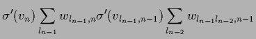
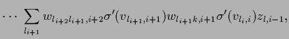
In particular, the stationarity equation for functional (352)
becomes
.
In particular, the stationarity equation for functional (352)
becomes
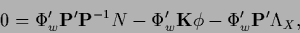 |
(417) |
with matrix of derivatives
and
 =
=  .
While
.
While  is calculated by forward propagating
 =
=  through the net defined by
weight vector
according to
Eq. (415) the derivatives
through the net defined by
weight vector
according to
Eq. (415) the derivatives
 can efficiently be calculated by back-propagation
according to Eq. (418).
Notice that even for diagonal
can efficiently be calculated by back-propagation
according to Eq. (418).
Notice that even for diagonal
 the derivatives are not needed only at data points
but the prior and normalization term require derivatives
at all , .
Thus, in practice terms like
the derivatives are not needed only at data points
but the prior and normalization term require derivatives
at all , .
Thus, in practice terms like
 have to be calculated in a relatively poor discretization.
Notice, however, that regularization is here
not only due to the prior term but
follows also from the restrictions implicit
in a chosen neural network architecture.
In many practical cases
a relatively poor discretization of the prior term may thus be sufficient.
have to be calculated in a relatively poor discretization.
Notice, however, that regularization is here
not only due to the prior term but
follows also from the restrictions implicit
in a chosen neural network architecture.
In many practical cases
a relatively poor discretization of the prior term may thus be sufficient.
Table 6 summarizes the discussed approaches.
Table 6:
Some possible parameterizations.
| Ansatz |
Functional form |
to be optimized |
| linear ansatz |
 |
 |
| linear model |
 |
 , , |
 with interaction with interaction |
 |
 |
| mixture model |
 |
 , , |
| additive model |
 |
 |
| with interaction |
 |
 |
| product ansatz |
 |
|
| decision trees |
 |
,  , ,  |
| projection pursuit |
 |
, , , |
| neural net (2 lay.) |
 |
, |
|
Next: Parameterizing priors: Hyperparameters
Up: Parameterizing likelihoods: Variational methods
Previous: Projection pursuit
Contents
Joerg_Lemm
2001-01-21