Next: Equal covariances
Up: Prior mixtures
Previous: Analytical solution
Contents
Low and high temperature limits
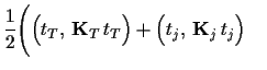
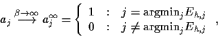
are extremely useful because in both cases
the stationarity Eq.(21) becomes linear,
corresponding thus to
classical quadratic regularisation approaches.
In the high temperature limit
 the exponential factors
  become
  -independent
 |
(34) |
(for
 replace
  by
by
 ).
The solution
).
The solution
 is a (generalised) `complete template average'
 |
(35) |
with
 |
(36) |
This high temperature solution
corresponds to the minimum of the quadratic
functional
 ,
,
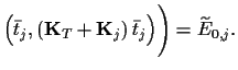
In the low temperature limit
 only the maximal component contributes,
i.e.,
only the maximal component contributes,
i.e.,
 |
(37) |
(for  replace
  by
by
 )
assuming
)
assuming
 =
=  +
+  or
= +
or
= +  +
+
 .
Hence,
low temperature solutions
.
Hence,
low temperature solutions
 ,
are
all (generalised) `component averages'
,
are
all (generalised) `component averages'
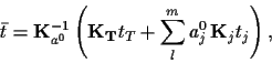
 provided they
fulfil the stability condition
provided they
fulfil the stability condition
 |
(38) |
or, after
performing a (generalised) `bias-variance' decomposition,
 ,
with
,
with
 matrices
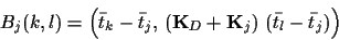 |
(39) |
and (generalised) `template variances'
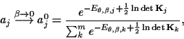
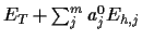
That means
single component averages
(which minimise and thus
 )
become solutions at zero temperature
)
become solutions at zero temperature  in case their (generalised) variance
  measuring the discrepancy between data and prior term is small
enough.
measuring the discrepancy between data and prior term is small
enough.
Next: Equal covariances
Up: Prior mixtures
Previous: Analytical solution
Contents
Joerg_Lemm
1999-12-21