Next: Initial configurations and kernel
Up: Learning matrices
Previous: Inverting in subspaces
Contents
For a differential operator
invertability can be achieved
by adding an operator
restricted to a subset
 (boundary).
More general, we consider an projector
(boundary).
More general, we consider an projector
 on a space which we will call boundary
and the projector on the interior
on a space which we will call boundary
and the projector on the interior  =
=
 .
We write
.
We write
 =
=
 for
for  ,
and require
,
and require
 .
That means
.
That means  is not symmetric,
but
is not symmetric,
but
 can be,
and we have
can be,
and we have
 |
(668) |
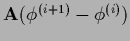
For such an
an equation of the form
 can be decomposed into
with projected
 ,
,
 ,
so that
,
so that
The boundary part is independent of the interior,
however, the interior can depend on the boundary.
A basis can be chosen so that the projector onto the boundary is diagonal,
i.e.,
Eliminating the boundary
results in an equation for the interior
with adapted inhomogeneity.
The special case
 =
=  ,
i.e.,
,
i.e.,  on the boundary,
is known as Dirichlet boundary conditions.
on the boundary,
is known as Dirichlet boundary conditions.
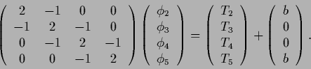
As trivial example of an equation  =
=  with boundary conditions,
consider a one-dimensional finite difference approximation
for a negative Laplacian
with boundary conditions,
consider a one-dimensional finite difference approximation
for a negative Laplacian  ,
adapted to include boundary conditions
as in Eq. (668),
,
adapted to include boundary conditions
as in Eq. (668),
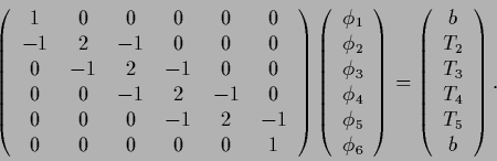 |
(673) |
Then Eq. (669)
is equivalent to the boundary conditions,
 =
=  ,
,  = ,
and the interior equation Eq. (670) reads
= ,
and the interior equation Eq. (670) reads
 |
(674) |
(Useful references dealing with the
numerical solution of partial differential equations are, for example,
[8,161,87,196,84].)
Similarly to boundary conditions for ,
we may use a learning matrix  with boundary conditions
(corresponding for example to those used for ):
with boundary conditions
(corresponding for example to those used for ):
For linear  the form (675)
corresponds to general linear boundary conditions.
(It is also possible to require nonlinear boundary conditions.)
the form (675)
corresponds to general linear boundary conditions.
(It is also possible to require nonlinear boundary conditions.)
 can be chosen symmetric,
and therefore positive definite,
and the boundary of can
be changed during iteration.
Solving
can be chosen symmetric,
and therefore positive definite,
and the boundary of can
be changed during iteration.
Solving
 =
=
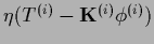 gives on the boundary and for the interior
 |
(677) |
 |
(678) |
For fulfilled boundary conditions with
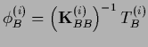 and
and
 ,
or for
,
or for
 so the boundary is not updated,
the term
so the boundary is not updated,
the term
 vanishes.
Otherwise, inserting the first in the second equation gives
vanishes.
Otherwise, inserting the first in the second equation gives
Even if is not defined with boundary conditions,
an invertible can be obtained from
by introducing a boundary for .
The updating process is then
restricted to the interior.
In such cases the boundary should be systematically changed
during iteration.
Block-wise updating of  represent a special case
of such learning matrices with variable boundary.
represent a special case
of such learning matrices with variable boundary.
The following table summarizes the learning matrices
we have discussed in some detail for the setting of density estimation
(for conjugate gradient and quasi-Newton methods
see, for example, [196]):
| Learning algorithm |
Learning matrix |
| Gradient |
 |
| Jacobi |
 |
| Gauss-Seidel |
 |
| Newton |
 |
| prior relaxation |
 |
| massive relaxation |
 |
| linear boundary |
 |
| Dirichlet boundary |
 |
| Gaussian |
 |
Next: Initial configurations and kernel
Up: Learning matrices
Previous: Inverting in subspaces
Contents
Joerg_Lemm
2001-01-21