


Next: Boundary conditions
Up: Learning matrices
Previous: Gaussian relaxation
Contents
Matrices considered as learning matrix
have to be invertible.
Non-invertible matrices can only be inverted in
the subspace which is the complement of its zero space.
With respect to a symmetric
 we define
the projector
we define
the projector
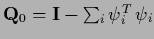 into its zero space
(for the more general case of a normal
replace
into its zero space
(for the more general case of a normal
replace  by the hermitian conjugate
 )
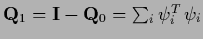
and its complement
)
and its complement
 with
with  denoting orthogonal eigenvectors with eigenvalues
  of , i.e.,
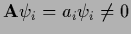 .
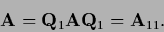
Then, denoting projected sub-matrices by
.
Then, denoting projected sub-matrices by
 =
=  we have
 =
=  =
=  =
=  ,
i.e.,
,
i.e.,
 |
(660) |
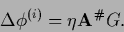
and in the update equation
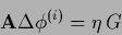 |
(661) |
only  can be inverted.
Writing
can be inverted.
Writing
 =
=  for a projected vector,
the iteration scheme acquires the form
for a projected vector,
the iteration scheme acquires the form
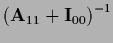
For positive semi-definite
the sub-matrix is positive definite.
If the second equation is already fulfilled
or its solution is postponed to a later iteration step we have
In case the projector
 is diagonal in the chosen representation
the projected equation
can directly be solved by skipping the corresponding components.
Otherwise one can use the Moore-Penrose inverse
is diagonal in the chosen representation
the projected equation
can directly be solved by skipping the corresponding components.
Otherwise one can use the Moore-Penrose inverse  of to
solve the projected equation
of to
solve the projected equation
 |
(666) |
Alternatively, an invertible operator
 can be added to to obtain a complete iteration scheme
with
can be added to to obtain a complete iteration scheme
with  =
=
 +
+

The choice
=
 =
=
 ,
=
,
=
 ,
for instance,
results in a gradient algorithm on the zero space
with additional coupling between the two subspaces.
,
for instance,
results in a gradient algorithm on the zero space
with additional coupling between the two subspaces.
Next: Boundary conditions
Up: Learning matrices
Previous: Gaussian relaxation
Contents
Joerg_Lemm
2001-01-21