A priori information and a posteriori control

Learning is based on data, which includes training data as well as a priori data. It is prior knowledge which, besides specifying the space of local hypothesis, enables generalization by providing the necessary link between measured training data and not yet measured or non-training data. The strength of this connection may be quantified by the mutual information of training and non-training data, as we did in Section 2.1.5.

Often, the role of a priori information seems to be underestimated. There are theorems, for example, proving that asymptotically learning results become independent of a priori information if the number of training data goes to infinity. This, however, is correct only if the space of hypotheses

is already sufficiently restricted and if a priori information means knowledge in addition to that restriction.

In particular, let us assume that the number of potential test situations

, is larger than the number of training data one is able to collect. As the number of actual training data has to be finite, this is always the case if

can take an infinite number of values, for example if

is a continuous variable. The following arguments, however, are not restricted to situations were one considers an infinite number of test situations, we just assume that their number is too large to be completely included in the training data.

If there are

values for which no training data are available, then learning for such

must refer to the mutual information of such test data and the available training data. Otherwise, training would be useless for these test situations. This also means, that the generalization to non-training situations can be arbitrarily modified by varying a priori information.

To make this point very clear, consider the rather trivial situation of learning a deterministic function

for a

variable which can take only two values

and

, from which only one can be measured. Thus, having measured for example

= 5, then ``learning''

is not possible without linking it to

. Such prior knowledge may have the form of a ``smoothness'' constraint, say $\vert h(x_1)-h(x_2)\vert\le 2$ which would allow a learning algorithm to ``generalize'' from the training data and obtain $3\le h(x_2)\le 7$ . Obviously, arbitrary results can be obtained for

by changing the prior knowledge. This exemplifies that generalization can be considered as a mere reformulation of available information, i.e., of training data and prior knowledge. Except for such a rearrangement of knowledge, a learning algorithm does not add any new information to the problem. (For a discussion of the related ``no-free-lunch'' theorems see [240,241].)

Being extremely simple, this example nevertheless shows a severe problem. If the result of learning can be arbitrary modified by a priori information, then it is critical which prior knowledge is implemented in the learning algorithm. This means, that prior knowledge needs an empirical foundation, just like standard training data have to be measured empirically. Otherwise, the result of learning cannot expected to be of any use.

Indeed, the problem of appropriate a priori information is just the old induction problem, i.e., the problem of learning general laws from a finite number of observations, as already been discussed by the ancient Greek philosophers. Clearly, this is not a purely academic problem, but is extremely important for every system which depends on a successful control of its environment. Modern applications of learning algorithms, like speech recognition or image understanding, rely essentially on correct a priori information. This holds especially for situations where only few training data are available, for example, because sampling is very costly.

Empirical measurement of a priori information, however, seems to be impossible. The reason is that we must link every possible test situation to the training data. We are not able to do this in practice if, as we assumed, the number of potential test situations is larger than the number of measurements one is able to perform.

Take as example again a deterministic learning problem like the one discussed above. Then measuring a priori information might for example be done by measuring (e.g., bounds on) all differences

. Thus, even if we take the deterministic structure of the problem for granted, the number of such differences is equal to the number of potential non-training situations

we included in our model. Thus, measuring a priori information does not require fewer measurements than measuring directly all potential non-training data. We are interested in situations where this is impossible.

Going to a probabilistic setting the problem remains the same. For example, even if we assume Gaussian hypotheses with fixed variance, measuring a complete mean function

, say for continuous

, is clearly impossible in practice. The same holds thus for a Gaussian process prior on

. Even this very specific prior requires the determination of a covariance and a mean function (see Chapter 3).

As in general empirical measurement of a priori information seems to be impossible, one might thus just try to guess some prior. One may think, for example, of some ``natural'' priors. Indeed, the term ``a priori'' goes back to Kant [111] who assumed certain knowledge to be necessarily be given ``a priori'' without reference to empirical verification. This means that we are either only able to produce correct prior assumptions, for example because incorrect prior assumptions are ``unthinkable'', or that one must typically be lucky to implement the right a priori information. But looking at the huge number of different prior assumptions which are usually possible (or ``thinkable''), there seems no reason why one should be lucky. The question thus remains, how can prior assumptions get empirically verified.

Also, one can ask whether there are ``natural'' priors in practical learning tasks. In Gaussian regression one might maybe consider a ``natural'' prior to be a Gaussian process with constant mean function and smoothness-related covariance. This may leave a single regularization parameter to be determined for example by cross-validation. Formally, one can always even use a zero mean function for the prior process by subtracting a base line or reference function. Thus does, however, not solve the problem of finding a correct prior, as now that reference function has to be known to relate the results of learning to empirical measurements. In principle any function could be chosen as reference function. Such a reference function would for example enter a smoothness prior. Hence, there is no ``natural'' constant function and from an abstract point of view no prior is more ``natural'' than any other.

Formulating a general law refers implicitly (and sometimes explicitly) to a ``ceteris paribus'' condition, i.e., the constraint that all relevant variables, not explicitly mentioned in the law, are held constant. But again, verifying a ``ceteris paribus'' condition is part of an empirical measurement of a priori information and by no means trivial.

Trying to be cautious and use only weak or ``uninformative'' priors does also not solve the principal problem. One may hope that such priors (which may be for example an improper constant prior for a one-dimensional real variable) do not introduce a completely wrong bias, so that the result of learning is essentially determined by the training data. But, besides the problem to define what exactly an uninformative prior has to be, such priors are in practice only useful if the set of possible hypothesis is already sufficiently restricted, so ``the data can speak for themselves'' [69]. Hence, the problem remains to find that priors which impose the necessary restrictions, so that uninformative priors can be used.

Hence, as measuring a priori information seems impossible and finding correct a priori information by pure luck seems very unlikely, it looks like also successful learning is impossible. It is a simple fact, however, that learning can be successful. That means there must be a way to control a priori information empirically.

Indeed, the problem of measuring a priori information may be artificial, arising from the introduction of a large number of potential test situations and correspondingly a large number of hidden variables

(representing what we call ``Nature'') which are not all observable.

In practice, the number of actual test situations is also always finite, just like the number of training data has to be. This means, that not all potential test data but only the actual test data must be linked to the training data. Thus, in practice it is only a finite number of relations which must be under control to allow successful generalization. (See also Vapnik's distinction between induction and transduction problems. [226]: In induction problems one tries to infer a whole function, in transduction problems one is only interested in predictions for a few specific test situations.)

This, however, opens a possibility to control a priori information empirically. Because we do not know which test situation will occur, such an empirical control cannot take place at the time of training. This means a priori information has to be implemented at the time of measuring the test data. In other words, a priori information has to be implemented by the measurement process [132,135].

Again, a simple example may clarify this point. Consider the prior information, that a function

is bounded, i.e., $a\le h(x)\le b$ , $\forall x$ . A direct measurement of this prior assumption is practically not possible, as it would require to check every value

. An implementation within the measurement process is however trivial. One just has to use a measurement device which is only able to to produce output in the range between

and

. This is a very realistic assumption and valid for all real measurement devices. Values smaller than

and larger than

have to be filtered out or actively projected into that range. In case we nevertheless find a value out of that range we either have to adjust the bounds or we exchange the ``malfunctioning'' measurement device with a proper one. Note, that this range filter is only needed at the finite number of actual measurements. That means, a priori information can be implemented by a posteriori control at the time of testing.

A realistic measurement device does not only produce bounded output but shows also always input noise or input averaging. A device with input noise has noise in the

variable. That means if one intends to measure at

the device measures instead at $x_i+\Delta$ with $\Delta$ being a random variable. A typical example is translational noise, with $\Delta$ being a, possibly multidimensional, Gaussian random variable with mean zero. Similarly, a device with input averaging returns a weighted average of results for different

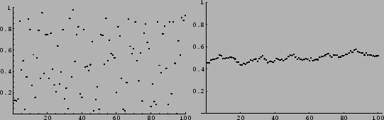
values instead of a sharp result. Bounded devices with translational input noise, for example, will always measure smooth functions [129,23,132]. (See Fig. 4.) This may be an explanation for the success of smoothness priors.

**Figure 4:** The l.h.s. shows a bounded random function which does not allow generalization from training to non-training data. Using a measurement device with input averaging (r.h.s.) or input noise the function becomes learnable.
$\begin{figure}\epsfig{file=ps/orgpic.eps, width=60mm}\epsfig{file=ps/avpic.eps, width=60mm}\end{figure}$

The last example shows, that to obtain adequate a priori information it can be helpful in practice to analyze the measurement process for which learning is intended. The term ``measurement process'' does here not only refer to a specific device, e.g., a box on the table, but to the collection of all processes which lead to a measurement result.

We may remark that measuring a measurement process is as difficult or impossible as a direct measurement of a priori information. What has to be ensured is the validity of the necessary restrictions during a finite number of actual measurements. This is nothing else than the implementation of a probabilistic rule producing

given the test situation and the training data. In other words, what has to be implemented is the predictive density $p(y\vert x,D)$ . This predictive density indeed only depends on the actual test situation and the finite number of training data. (Still, the probability density for a real

cannot strictly be empirically verified or controlled. We may take it here, for example, as an approximate statement about frequencies.) This shows the tautological character of learning, where measuring a priori information means controlling directly the corresponding predictive density.

The a posteriori interpretation of a priori information can be related to a constructivistic point of view. The main idea of constructivism can be characterized by a sentence of Vico (1710): Verum ipsum factum -- the truth is the same as the made [227]. (For an introduction to constructivism see [232] and references therein, for constructive mathematics see [25].)