


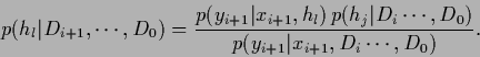
Next: Bayesian decision theory
Up: Basic model and notations
Previous: Predictive density
Contents
Mutual information and learning
The aim of learning is to generalize
the information obtained from training data to non-training situations.
For such a generalization to be possible,
there must exist a, at least partially known,
relation between the likelihoods  for training and for non-training data.
This relation is typically provided by a priori knowledge.
for training and for non-training data.
This relation is typically provided by a priori knowledge.
One possibility to quantify
the relation between two random variables  and
and  ,
representing for example training and non-training data,
is to calculate their mutual information,
defined as
,
representing for example training and non-training data,
is to calculate their mutual information,
defined as
 |
(28) |
It is also instructive to express the mutual information
in terms of (average) information content or entropy,
which, for a probability function  , is defined as
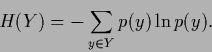 |
(29) |
We find
 |
(30) |
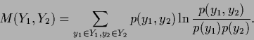
meaning that the mutual information
is the sum of the two individual entropies
diminished by the entropy common to both variables.
To have a compact notation
for a family of predictive densities
 we choose a vector
 =
=
 consisting of all possible values
  and corresponding vector
 =
=
 ,
so we can write
,
so we can write
 |
(31) |
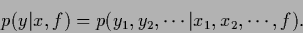
We now would like to characterize a state of knowledge  corresponding to predictive density
  by its mutual information.
Thus, we generalize
the definition (28) from two random variables
to a random vector with components
by its mutual information.
Thus, we generalize
the definition (28) from two random variables
to a random vector with components  ,
given vector with components
and obtain the conditional mutual information
,
given vector with components
and obtain the conditional mutual information
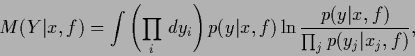 |
(32) |
or
 |
(33) |
in terms of conditional entropies
 |
(34) |
In case not a fixed vector is given,
like for example =
,
but a density  ,
it is useful to average
the conditional mutual information and
conditional entropy
by including the integral
,
it is useful to average
the conditional mutual information and
conditional entropy
by including the integral
 in the above formulae.
It is clear from Eq. (32)
that predictive densities
which factorize
 |
(35) |
have a mutual information of zero.
Hence,
such factorial states
do not allow any generalization from training to non-training data.
A special example are the possible states of Nature or
pure states  ,
which factorize according to the definition of our model
,
which factorize according to the definition of our model
 |
(36) |
Thus, pure states do not allow any further generalization.
This is consistent with the fact that
pure states represent the natural endpoints of any learning process.
It is interesting to see, however,
that there are also other states for which the predictive
density factorizes.
Indeed, from Eq. (36) it follows that
any (prior or posterior) probability  which factorizes leads to a factorial state,
 |
(37) |
This means generalization, i.e., (non-local) learning,
is impossible when starting from a factorial prior.
A factorial prior provides a very clear reference
for analyzing the role of a-priori information in learning.
In particular, with respect to a prior
factorial in local variables ,
learning may be decomposed into two steps, one increasing,
the other lowering mutual information:
- 1.
- Starting from a factorial prior,
new non-local data
 (typically called a priori information)
produce a new non-factorial state
with non-zero mutual information.
(typically called a priori information)
produce a new non-factorial state
with non-zero mutual information.
- 2.
- Local data
 (typically called training data)
stochastically
reduce the mutual information.
Hence, learning with local data corresponds to a
stochastic decay of mutual information.
(typically called training data)
stochastically
reduce the mutual information.
Hence, learning with local data corresponds to a
stochastic decay of mutual information.
Pure states,
i.e., the extremal points in the space of possible predictive densities,
do not have to be deterministic.
Improving measurement devices,
stochastic pure states
may be further decomposed into finer components  , so that
 |
(38) |
Imposing a non-factorial prior  on the new, finer hypotheses
enables again non-local learning with local data,
leading asymptotically
to one of the new pure states
on the new, finer hypotheses
enables again non-local learning with local data,
leading asymptotically
to one of the new pure states  .
.
Let us exemplify
the stochastic decay of mutual information
by a simple numerical example.
Because the mutual information requires
the integration over all variables
we choose a problem with only two of them,
 and
and  corresponding to
two values
corresponding to
two values  and
and  .
We consider a model with four
states of Nature
.
We consider a model with four
states of Nature  ,
,  ,
with Gaussian likelihood
,
with Gaussian likelihood
 =
=
 and local means
  =
=  .
.
Selecting a ``true'' state of Nature ,
we sample 50 data points  =
=  from the corresponding Gaussian likelihood
using
from the corresponding Gaussian likelihood
using  =
=  =
=  .
Then, starting from a given, factorial or non-factorial, prior
.
Then, starting from a given, factorial or non-factorial, prior
 we sequentially update the predictive density,
 |
(39) |
by calculating the posterior
 |
(40) |
It is easily seen from Eq. (40)
that factorial states remain factorial under local data.
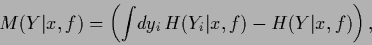
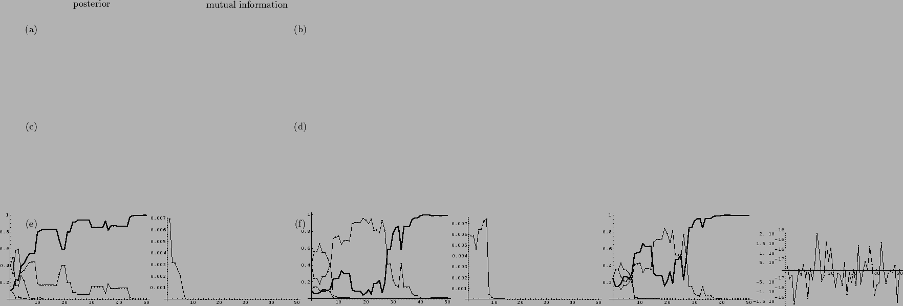
Fig. 3 shows that indeed the mutual information decays rapidly.
Depending on the training data,
still the wrong hypothesis may survive
the decay of mutual information.
Having arrived at a factorial state,
further learning has to be local.
That means, data points for
can then only influence the predictive density for the corresponding
and do not allow generalization to the other  with
with  .
.
For a factorial prior
 =
=
 learning is thus local from the very beginning.
Only very small numerical random fluctuations of the mutual information
occur, quickly eliminated by learning.
Thus, the predictive density
moves through a sequence of factorial states.
learning is thus local from the very beginning.
Only very small numerical random fluctuations of the mutual information
occur, quickly eliminated by learning.
Thus, the predictive density
moves through a sequence of factorial states.
Figure 3:
The decay of mutual information during learning:
Model with 4 possible states
representing Gaussian likelihoods
 with means for two different values.
Shown are posterior probabilities
with means for two different values.
Shown are posterior probabilities
 (
( ,
,  ,
,  , on the left hand side,
the posterior of the true is shown by a thick line)
and mutual information
, on the left hand side,
the posterior of the true is shown by a thick line)
and mutual information  (
( ,
,  , , on the right hand side)
during learning 50 training data.
(, ): The mutual information decays during learning
and becomes quickly practically zero.
(, ): For ``unlucky'' training data
the wrong hypothesis
, , on the right hand side)
during learning 50 training data.
(, ): The mutual information decays during learning
and becomes quickly practically zero.
(, ): For ``unlucky'' training data
the wrong hypothesis  can dominate at the beginning.
Nevertheless, the mutual information decays and
the correct hypothesis has finally to be found through
``local'' learning.
(, ): Starting with a factorial prior
the mutual information is and remains zero,
up to artificial numerical fluctuations.
For (, ) the same random data
have been used as for (, ).
can dominate at the beginning.
Nevertheless, the mutual information decays and
the correct hypothesis has finally to be found through
``local'' learning.
(, ): Starting with a factorial prior
the mutual information is and remains zero,
up to artificial numerical fluctuations.
For (, ) the same random data
have been used as for (, ).
 |
Next: Bayesian decision theory
Up: Basic model and notations
Previous: Predictive density
Contents
Joerg_Lemm
2001-01-21