An implicit method

One can try to overcome the problems with conditional stability by introducing an implicit scheme. The simplest way to do it is just to replace all terms on the right hand side of (2.9) by an average from the values to the time steps $j+1$ and $j-1$ , i.e,

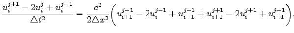$$\frac{u_i^{j+1}-2u_i^j+u_i^{j-1}}{\triangle t^2}=\frac{c^2}{2\tri... ...}^{j-1}-2u_i^{j-1}+u_{i-1}^{j-1}+u_{i+1}^{j+1}-2u_i^{j+1}+u_{i-1}^{j+1}\biggr).$$ (2.13)

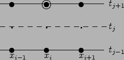
The schematical diagramm of the scheme (2.13) is schown on Fig. (2.1.2 )

Figure 2.2: Schematical visualization of the implicit numerical scheme (2.13) for (2.2).

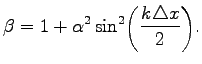
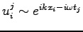
Let us check the stability of (2.13). To this aim we use the standart ansatz

$$\varepsilon_i^{j+1}=g^{j}e^{ikx_i}$$

leading to the equation for $g(k)$

$$\beta g^2-2g+\beta=0$$

with

$$\beta=1+\alpha^2\sin^2\biggl(\frac{k\triangle x}{2}\biggr).$$

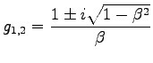
One can see that $\beta\geq1$ for all $k$ . Hence the solutions $g_{1,2}$ take the form

$$g_{1,2}=\frac{1\pm i\sqrt{1-\beta^2}}{\beta}$$

and

$$\vert g\vert^2=\frac{1-(1-\beta^2)}{\beta^2}=1.$$

Hence, the scheme (2.13) is absolute stable.

The question now is, whether the implicit scheme (2.13) is better than the explicit scheme (2.10) form numerical point of view. To answer this question, let us analyse dispersion relation for Eq. (2.2) as well as for both schemes (2.10) and (2.13). Exact dispersion relation is

$$\omega=\pm ck,$$

i.e, all Fourier modes propagate without dispersion with the same phase velocity $\omega/k=\pm c$ .

Using the ansatz $u_i^j\sim e^{ikx_i-i\omega t_j}$ for the explicit method (2.10) one obtains:

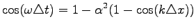$$\cos(\omega\triangle t)=1-\alpha^2(1-\cos(k\triangle x))$$ (2.14)

while for the implicit method (2.13)

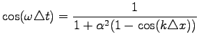$$\cos(\omega\triangle t)=\frac{1}{1+\alpha^2(1-\cos(k\triangle x))}$$ (2.15)

Figure 2.3: Dispersion relation for the explicit (blue curves) and implicit (red curves) methods.

One can see that for $\alpha\rightarrow 0$ both methods provide the same result, otherwise the explicit scheme always exceeds the implicit one (see Fig. (2.1.2)). For $\alpha=1$ the scheme (2.10) becomes exact, while (2.13) deviates more and more from the exact value of $\omega$ for increasing $\alpha$ . Hence, there are no motivation to use implicit scheme instead of the explicit one.