An explicit method

The first idea is just to use central differences for both time and space derivatives, i.e.,

$$\frac{u_i^{j+1}-2u_i^j+u_i^{j-1}}{\triangle t^2}=c^2\frac{u_{i+1}^{j}-2u_i^j+u_{i-1}^{j}}{\triangle x^2}$$ (2.9)

or, with $\alpha=c\triangle t/\triangle x$

$$\boxed{u_i^{j+1}=-u_i^{j-1}+2(1-\alpha^2)u_i^{j}+\alpha^2(u_{i+1}^j+u_{i-1}^j)}$$ (2.10)

Schematical representation of the scheme can be seen on Fig. 2.1.2.

Figure 2.1: Schematical visualization of the numerical scheme (2.10) for (2.2).

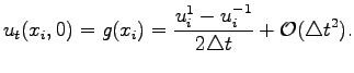
Besides, one should add the initial conditions (2.7). To the implementation of the second initial condition one needs again the virtual point $u_i^{-1}$ ,

$$u_t(x_i,0)=g(x_i)=\frac{u_i^1-u_i^{-1}}{2\triangle t}+\mathcal{O}(\triangle t^2).$$

With $g_i:=g(x_i)$ one can rewrite the last expression as

$$u_i^{-1}=u_i^1-2\triangle t g_i+\mathcal{O}(\triangle t^2),$$

and the second time row can be calculated as

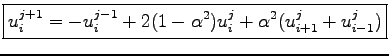
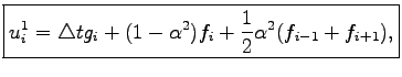
$$\boxed{u_i^1=\triangle tg_i+(1-\alpha^2)f_i+\frac{1}{2}\alpha^2(f_{i-1}+f_{i+1}),}$$ (2.11)

where $u(x_i,0)=u_i^0=f(x_i)=f_i$ .