Let ![]() be the cube circumscribed to the reconstruction region
be the cube circumscribed to the reconstruction region ![]() with edges parallel to the coordinate axes and aligned with the direction
with edges parallel to the coordinate axes and aligned with the direction ![]() of the j-th incoming wave. Let
of the j-th incoming wave. Let ![]() be the face lying in the plane
be the face lying in the plane ![]() , and let
, and let ![]() be the other faces of
be the other faces of ![]() . Rather than working with the scattered fields
. Rather than working with the scattered fields ![]() we use the scaled scattered fields
we use the scaled scattered fields ![]() which satisfy
which satisfy
Note that we do not make the parabolic approximation [8], i.e. we do not assume that the second derivative of ![]() in direction
in direction ![]() is small compared to
is small compared to ![]() .
.
In [12] we haved analysed the stability of the initial value problem
for this elliptic differential equation. Let
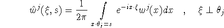
be the 2D Fourier transform of w in the plane ![]() . We found that
. We found that ![]() depends in a perfectly stable way on the initial values for
depends in a perfectly stable way on the initial values for ![]() on
on ![]() for all frequencies
for all frequencies ![]() where
where ![]() is some number depending
essentially on k and, to a minor extent, on f. In ultrasound tomography we can choose
is some number depending
essentially on k and, to a minor extent, on f. In ultrasound tomography we can choose ![]() slightly smaller than k, typically
slightly smaller than k, typically ![]() .
.
Thus we may define a nonlinear map ![]() by
putting
by
putting
The inverse scattering problem now calls for the solution of the nonlinear system
As in [12] this is done by an ART-type procedure. Starting out from an initial approximation ![]() , we put
, we put ![]() and for
and for ![]()
![]()
The first approximation ![]() is then defined to be
is then defined to be ![]() . For
. For ![]() we simply take the operator
we simply take the operator ![]() where
where ![]() is chosen such that, in the limit
is chosen such that, in the limit ![]() ,
,
![]() , i.e.
, i.e. ![]() [10]. The
evaluation of
[10]. The
evaluation of ![]() for some
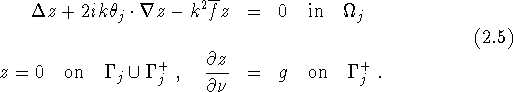
for some ![]() can be done as follows: Solve the initial value problem
can be done as follows: Solve the initial value problem
Then,
![]()
where ![]() is the solution of (2.1) - (2.2). Of course the stability properties of (2.5) are exactly as discussed above.
is the solution of (2.1) - (2.2). Of course the stability properties of (2.5) are exactly as discussed above.