

Next: Gaussian regression
Up: Mixtures of Gaussian process
Previous: Introduction
Contents
The Bayesian model
Let us consider
the following random variables:
- 1.
 , representing (a vector of)
independent, visible variables (`measurement situations'),
- 2.
 , being (a vector of)
dependent, visible variables (`measurement results'),
and
- 3.
 , being the hidden variables (`possible states of Nature').
A Bayesian approach is based on two model inputs
[1,11,4,12]:
- 1.
- A likelihood model
 ,
describing the density of observing
  given
given  and
and  .
Regarded as function of
  , for fixed
  and
and  ,
the density
  is also known as the (
 -conditional) likelihood of
  .
.
- 2.
- A prior model
 , specifying
the a priori density of
  given some a priori information denoted by
  (but before training data
  have been taken into account).
Furthermore,
to decompose a possibly complicated prior density
into simpler components,
we introduce
continuous hyperparameters  and discrete hyperparameters
  (extending the set of hidden variables to
  =
=  ),
),
 |
(1) |
In the following, the summation
over  will be treated exactly,
while the
  -integral will
be approximated.
A Bayesian approach aims in calculating the predictive density
for outcomes
  in test situations
 |
(2) |
given data  =
=  consisting of
a priori data
  and
i.i.d. training data
  =
=
 .
The vector of all
  (
( )
will be denoted
 .
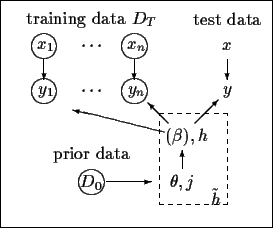
Fig.1 shows a graphical representation
of the considered probabilistic model.
In saddle point approximation
(maximum a posteriori approximation)
the  -integral becomes
 |
(3) |
 |
(4) |
assuming  to be slowly varying at the stationary point.
The posterior density is related to
(
 -conditional) likelihood and prior
according to Bayes' theorem
 |
(5) |
where the  -independent denominator (evidence)
can be skipped when maximising with respect to
  .
Treating the
  -integral within
  also in saddle point approximation
the posterior must be maximised
with respect to
  and
and  simultaneously .
Figure 1:
Graphical representation of
the considered probabilistic model,
factorising according to
 =
=


 .
(The variable
  is introduced
in Section 3.)
Circles indicate visible variables.
 |


Next: Gaussian regression
Up: Mixtures of Gaussian process
Previous: Introduction
Contents
Joerg_Lemm
1999-12-21
![]() and discrete hyperparameters
and discrete hyperparameters ![]() (extending the set of hidden variables to
(extending the set of hidden variables to ![]() =
= ![]() ),
),

![]() -integral becomes
-integral becomes
