


Next: A numerical example
Up: Bayesian Field Theory Nonparametric
Previous: Basic definitions
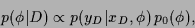
In this paper, our aim will be to reconstruct
the field  from observational data
  in Maximum A Posteriori Approximation (MAP),
i.e,
by maximizing
in Maximum A Posteriori Approximation (MAP),
i.e,
by maximizing
 |
(2) |
with respect to .
[Alternatively, one can use Monte-Carlo methods to approximate
the Bayesian predictive density  .]
Implementing the normalization conditions on
.]
Implementing the normalization conditions on  (for all
  )
by a Lagrange term with multiplier function
)
by a Lagrange term with multiplier function  ,
introducing an additional Gaussian process prior term for
[2]
(with zero mean and inverse covariance
,
introducing an additional Gaussian process prior term for
[2]
(with zero mean and inverse covariance  ,
real symmetric, positive definite),
and considering the usual case where the
positivity constraint is not active at the stationary point
(or automatically satisfied by the choice of )
so a corresponding Lagrange multiplier can be skipped,
we have therefore to minimize the error functional,
,
real symmetric, positive definite),
and considering the usual case where the
positivity constraint is not active at the stationary point
(or automatically satisfied by the choice of )
so a corresponding Lagrange multiplier can be skipped,
we have therefore to minimize the error functional,
 |
(3) |
Here
 denotes the empirical density, i.e.,
 =
=
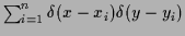 ,
and the bra-ket notation
,
and the bra-ket notation
 ,
denoting scalar products,
stands for integration over and
,
denoting scalar products,
stands for integration over and  .
(Thus, the error functional (3)
is, up to a -independent constant
and the constraint implementation by Lagrange multiplier terms,
the negative logarithm of the posterior (2).
Prior terms can be made more flexible by including hyperparameters
[1,6].
See [4] for a more detailed discussion.)
Notice that a Gaussian prior term in the field
is in general non-Gaussian in terms of the
conditional likelihood .
.
(Thus, the error functional (3)
is, up to a -independent constant
and the constraint implementation by Lagrange multiplier terms,
the negative logarithm of the posterior (2).
Prior terms can be made more flexible by including hyperparameters
[1,6].
See [4] for a more detailed discussion.)
Notice that a Gaussian prior term in the field
is in general non-Gaussian in terms of the
conditional likelihood .
The MAP equation to be solved
is easily found by setting the functional derivative
of (3) with respect
to  to zero, yielding,
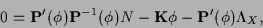 |
(4) |
where
 =
=
 and
and
 =
=
 .
For existing
.
For existing
 =
=
 this can be written
 |
(5) |
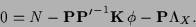
From the normalization condition
 =
=  [where
 =
=
 and
and
 =
=  ],
it follows for
],
it follows for
 =
=
 that
that
 =
=  ,
and thus, multiplying Eq. (5) by
,
and thus, multiplying Eq. (5) by  ,
,
 |
(6) |
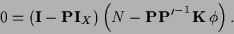
where
 =
=  =
=
 .
can now be eliminated by
inserting Eq. (6) into Eq. (5)
.
can now be eliminated by
inserting Eq. (6) into Eq. (5)
 |
(7) |
In contrast to regression
with Gaussian process priors [12]
(where MAP is exact),
and similarly, classification for a specific choice of  [11],
the solution of Eq. (7) cannot be found
in a finite dimensional space defined by the training data .
Thus,
Eq. (7) has to be solved by discretization,
analogously, for example, to solving
field theories on a lattice [7].
Starting with an initial guess
[11],
the solution of Eq. (7) cannot be found
in a finite dimensional space defined by the training data .
Thus,
Eq. (7) has to be solved by discretization,
analogously, for example, to solving
field theories on a lattice [7].
Starting with an initial guess  ,
a possible iteration scheme is given by
,
a possible iteration scheme is given by
![\begin{displaymath}
\phi^{(r+1)} =
\phi^{(r)} + \eta^{(r)} \left({\bf A}^{(r)}\...
...e}^{(r)}\right)^{-1}{{\bf K}}\,
\phi^{(r}) \right)
\right]
,
\end{displaymath}](img84.png) |
(8) |
with some positive definite matrix  ,
and a number
,
and a number  , both possibly changing during the iteration.
A convenient
, both possibly changing during the iteration.
A convenient  -independent choice for
is often the inverse covariance .
(Quasi-Newton methods, for example, use
an -dependent , the standard gradient algorithm
corresponds to choosing for the identity matrix.)
For each calculated gradient,
the factor
-independent choice for
is often the inverse covariance .
(Quasi-Newton methods, for example, use
an -dependent , the standard gradient algorithm
corresponds to choosing for the identity matrix.)
For each calculated gradient,
the factor  can be determined
by a one-dimensional line search algorithm.
An iteration scheme similar to Eq. (8),
can be obtained using Eq. (4),
which then requires to adapt the Lagrange multiplier function
during iteration.
can be determined
by a one-dimensional line search algorithm.
An iteration scheme similar to Eq. (8),
can be obtained using Eq. (4),
which then requires to adapt the Lagrange multiplier function
during iteration.
Clearly, a direct discretization can only be useful
for low dimensional and variables
(say one- or two-dimensional, like time series or images).
Due to increasing computing capabilities, however,
many low-dimensional problems
are now directly solvable by discretization [3].
For variables or
living in higher dimensional spaces
additional approximations are necessary [4].
Next: A numerical example
Up: Bayesian Field Theory Nonparametric
Previous: Basic definitions
Joerg_Lemm
2000-09-12