


Next: Maximum A Posteriori Approximation
Up: Bayesian Field Theory Nonparametric
Previous: Bayesian Field Theory Nonparametric
A Bayesian approach to empirical learning problems
requires two main inputs [1,10]:
1. a (conditional) likelihood model
 representing the probability of measuring
  given (visible) condition
  and (hidden) state of Nature
  .
2. a prior model
.
2. a prior model
 encoding the a priori information available on .
We assume that the joint probability factorizes
according to
encoding the a priori information available on .
We assume that the joint probability factorizes
according to
 |
(1) |
Furthermore, we will consider  independent (training) data
 =
=
 .
Denoting by
.
Denoting by
 (
( ) the vector of the
  (
( ),
we assume
),
we assume
 =
=
 and
and
 =
=
 .
Different classes of likelihood functions define different problem types.
In the following we will be interested
in general density estimation problems [9],
the other problems listed in Tab. 1
being special cases thereof.
.
Different classes of likelihood functions define different problem types.
In the following we will be interested
in general density estimation problems [9],
the other problems listed in Tab. 1
being special cases thereof.
Within nonparametric approaches,
the function values  = itself,
specifying a state of Nature ,
are considered as the primary degrees of freedom,
their only constraint being the positivity and normalization
conditions for .
In particular, we will study in this paper
likelihoods
= itself,
specifying a state of Nature ,
are considered as the primary degrees of freedom,
their only constraint being the positivity and normalization
conditions for .
In particular, we will study in this paper
likelihoods  being functionals of
fields
being functionals of
fields  , i.e., =
  .
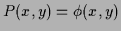
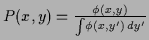
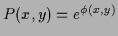
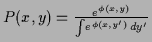
Examples of such functionals
are shown in Tab. 2.
While the first and third row show
the `local' functionals
corresponding to
= and
=
.
Examples of such functionals
are shown in Tab. 2.
While the first and third row show
the `local' functionals
corresponding to
= and
=  ,
the other functionals are nonlocal in .
,
the other functionals are nonlocal in .
Depending on the choice of the functional
the normalization and positivity constraint for
take different forms for .
For example, the normalization condition is automatically fulfilled
in rows two and four of Tab. 2.
In the last row, where
=
 ,
the normalization constraint for becomes the boundary condition
,
the normalization constraint for becomes the boundary condition
 = 1, and positivity of means monotony of
  .
.
Table 1:
Special cases of density estimation.
For classification and regression see
[12,11,3,4]
and references therein,
for clustering see [8], and
for Bayesian approaches to inverse quantum mechanics,
aiming for example in the reconstruction of potentials
from observational data, see [5].
( denotes the density operator of a quantum system,
 the projector to the eigenstate
of observable , represented by an hermitian operator,
with eigenvalue .)
the projector to the eigenstate
of observable , represented by an hermitian operator,
with eigenvalue .)
| (conditional) likelihood |
problem type |
| of general form |
density estimation |
| discrete |
classification |
![$\frac{1}{\sigma\sqrt{2\pi}}e^{-\frac{[y-\phi(x)]^2}{2\sigma^2}}$](img41.png) (Gaussian,
(Gaussian,  fixed) fixed) |
regression |
![$\sum_k\frac{1}{\sigma_k\sqrt{2\pi}}e^{-\frac{[y-\phi_k(x)]^2}{2\sigma_k^2}}$](img43.png) (mixture of Gaussians)
(mixture of Gaussians) |
clustering |
Trace(
 ) ) |
inverse quantum mechanics |
|
Table 2:
Constraints for some specific choices of
|
constraints |
 |
norm |
positivity |
 |
-- |
positivity |
 |
norm |
-- |
 |
-- |
-- |
 |
boundary |
monotony |
|
Next: Maximum A Posteriori Approximation
Up: Bayesian Field Theory Nonparametric
Previous: Bayesian Field Theory Nonparametric
Joerg_Lemm
2000-09-12