J. C. Lemm and J. Uhlig
Institut für Theoretische Physik I
Universität Münster, 48149 Münster, Germany
The reconstruction of inter-particle forces from observational data is of key importance for any application of quantum mechanics to real world systems. Such inverse problems have been studied intensively in inverse scattering theory and in inverse spectral theory for one-body systems in one and, later, in three dimensions [1,2]. In this Letter we now outline a method, designed to deal with inverse problems for many-body systems.
Inverse problems are notoriously ill-posed [3]. It is well known that for ill-posed problems additional a priori information is required to obtain a unique and stable solution. In this Letter we refer to a nonparametric Bayesian framework [4,5] where a priori information is implemented explicitly, i.e., in form of stochastic processes over potentials [6].
Calculating an exact solution is typically not feasible for inverse many-body problems. As an example of a possible approximation scheme we will study in the following an `Inverse Hartree-Fock Approximation' (IHFA). For situations where a Hartree-Fock (HF) ansatz is not sufficient, the inverse problem would have to be solved on top of other approximation schemes. A Random Phase Approximation or a full Time-Dependent Hartree-Fock Approximation [7,8,9,10], for example, would go beyond HF.
Bayesian methods can easily be adapted to different learning situations and have therefore been applied to a variety of empirical learning problems, including classification, regression, density estimation [11,12,13], and, recently, to quantum statistics [6]. In particular, using a Bayesian approach for quantum systems it is straightforward to deal with measurements of arbitrary quantum mechanical observables, to include classical noise processes, and to implement a priori information explicitly in terms of the potential.
Computationally, on the other hand, working with stochastic processes, or discretized versions thereof, is much more demanding than, for example, fitting a small number of parameters. This holds especially for applications to quantum mechanics where one cannot take full advantage of the convenient analytical features of Gaussian processes. Due to increasing computational resources, however, the corresponding learning algorithms become now numerically feasible.
To define the problem
let us consider many-fermion systems with Hamiltonians,
![]() =
= ![]() , consisting of a one-body part
, consisting of a one-body part ![]() (e.g., in coordinate space representation
(e.g., in coordinate space representation ![]() ,
with Laplacian
,
with Laplacian ![]() ,
mass
,
mass ![]() ,
, ![]() = 1),
and a two-body potential
= 1),
and a two-body potential ![]() .
Introducing fermionic creation and annihilation operators
.
Introducing fermionic creation and annihilation operators
![]() ,
, ![]() , corresponding to a complete
single particle basis
, corresponding to a complete
single particle basis
![]() ,
such Hamiltonians can be written,
,
such Hamiltonians can be written,
 |
(1) |
In order to apply the Bayesian framework we need two model inputs:
firstly, the probability ![]() of measuring the observational data
of measuring the observational data ![]() given a potential
given a potential ![]() (for fixed
(for fixed ![]() also known as likelihood of
also known as likelihood of ![]() ),
and, secondly,
a prior probability
),
and, secondly,
a prior probability ![]() for
for ![]() .
The probability for
.
The probability for ![]() given data
given data ![]() ,
also called the posterior probability for
,
also called the posterior probability for ![]() ,
is then obtained according to Bayes' rule,
,
is then obtained according to Bayes' rule,
As the first step,
we have to identify
the likelihood ![]() of
of ![]() for observational data
for observational data ![]() .
In order to be able to obtain information about the potential,
the system has to be prepared in a
.
In order to be able to obtain information about the potential,
the system has to be prepared in a ![]() -dependent state.
Such a state can be a stationary statistical state,
e.g. a canonical ensemble,
or a time-dependent state evolving according to the Hamiltonian
of the system.
In the following we will discuss many-body systems
prepared in their ground state
-dependent state.
Such a state can be a stationary statistical state,
e.g. a canonical ensemble,
or a time-dependent state evolving according to the Hamiltonian
of the system.
In the following we will discuss many-body systems
prepared in their ground state ![]() .
The (normalized)
.
The (normalized) ![]() -particle ground state wave function
-particle ground state wave function ![]() depends on
depends on ![]() and is antisymmetrized for fermions.
In particular,
we will study two kinds of observational data
and is antisymmetrized for fermions.
In particular,
we will study two kinds of observational data ![]() =
=
![]() :
(A)
:
(A) ![]() simultaneous measurements of the coordinates
of all
simultaneous measurements of the coordinates
of all ![]() particles,
(B)
particles,
(B) ![]() measurements of the coordinates of a single particle.
In case
measurements of the coordinates of a single particle.
In case ![]() ,
the
,
the ![]() th measurement results in a vector
th measurement results in a vector ![]() =
= ![]() ,
consisting of
,
consisting of ![]() components
components ![]() ,
each representing the coordinates of a single particle
(which may also form a vector, e.g., a three dimensional one).
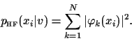
According to the axioms of quantum mechanics,
the probability of measuring
the coordinate vector
,
each representing the coordinates of a single particle
(which may also form a vector, e.g., a three dimensional one).
According to the axioms of quantum mechanics,
the probability of measuring
the coordinate vector ![]() , given
, given ![]() , is,
, is,
In contrast to an ideal measurement of a classical system,
the state of a quantum system is typically
changed by the measurement process.
In particular, its state is projected
in the space of eigenfunctions of the measured observable
with eigenvalue equal to the measurement result.
Hence, if we want to deal with
independent, identically distributed data,
the system must
be prepared in the same state before each measurement.
Under that condition the total likelihood factorizes
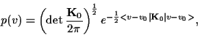
As the second step, we have to choose a prior probability ![]() .
A common and convenient choice are Gaussian prior probabilities
(or, for functions, Gaussian processes),
for which
.
A common and convenient choice are Gaussian prior probabilities
(or, for functions, Gaussian processes),
for which
Having defined
a likelihood ![]() for many-body quantum systems
and a prior probability
for many-body quantum systems
and a prior probability ![]() the next step is to solve the stationarity equation
for the posterior probability (2)
the next step is to solve the stationarity equation
for the posterior probability (2)
| (10) |
 |
(15) |
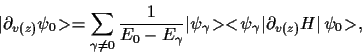
Again, we proceed by taking the derivative of
Eq. (12)
and obtain after standard manipulations
(for nondegenerate ![]() and
and
![]() = 0),
= 0),
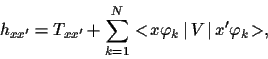
In conclusion,
reconstructing a potential from data by IHFA is based on
the definition of a prior probability
for ![]() and requires the iterative solution of
and requires the iterative solution of
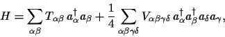
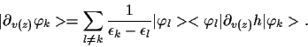
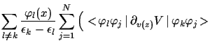
1. the stationarity equation for the potential (7), needing as input for each iteration step (21)
2. the derivatives of the likelihoods (19), obtained by solving the (two-body-like) equation (18) for given
3. single particle orbitals, defined in (12) as solutions of the direct (one-body) Hartree-Fock equation.
We tested the numerical feasibility
of the IHFA for a Hamiltonian
![]() =
= ![]() including a local two-body potential
including a local two-body potential ![]() to be reconstructed
and a local one-body potential
to be reconstructed
and a local one-body potential ![]() ,
with diagonal elements
,
with diagonal elements ![]() = 0 for
= 0 for ![]() and
and ![]() =
= ![]() elsewhere,
to confine the particles and
to break translational symmetry.
elsewhere,
to confine the particles and
to break translational symmetry.
To check the validity of the IHFA we must be able
to sample artificial data from
the exact true many-body likelihood (3)
for a given true potential ![]() .
Because this requires to solve the corresponding many-body problem exactly,
we have chosen a two-particle system
with one-dimensional
.
Because this requires to solve the corresponding many-body problem exactly,
we have chosen a two-particle system
with one-dimensional ![]() (on a grid with 21 points,
(on a grid with 21 points, ![]() = 10)
for which the true ground state can be calculated
by diagonalizing
= 10)
for which the true ground state can be calculated
by diagonalizing ![]() numerically.
We want to stress, however, that, in the case of real data,
application of the IHFA to systems with
numerically.
We want to stress, however, that, in the case of real data,
application of the IHFA to systems with ![]() particles is straightforward
and only requires to solve Eq. (18) for
particles is straightforward
and only requires to solve Eq. (18) for ![]() instead for two orbitals.
instead for two orbitals.
We selected a local true two-body potential ![]() with diagonal elements
with diagonal elements
![]() =
=
![]() and parameter values
(
and parameter values
(![]() = 1,
= 1, ![]() = 10,
= 10, ![]() =
= ![]() = 21 for mass
= 21 for mass ![]() =
= ![]() )
for which the iteration of the HF equation (12) converges.
(For two-body systems the HF iteration leads easily to oscillations.)
Calculating the true ground state
)
for which the iteration of the HF equation (12) converges.
(For two-body systems the HF iteration leads easily to oscillations.)
Calculating the true ground state ![]() for
for ![]() and the corresponding true likelihoods
(3) and (4)
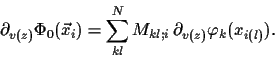
we then sampled:
(A)
and the corresponding true likelihoods
(3) and (4)
we then sampled:
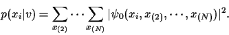
(A) ![]() = 100 two-particle data
from the true likelihood (3)
and
(B)
= 100 two-particle data
from the true likelihood (3)
and
(B) ![]() = 200 single particle data
from the true likelihood (4).
(See Figs. 1a and 2a.)
= 200 single particle data
from the true likelihood (4).
(See Figs. 1a and 2a.)
The calculations have been done for a Gaussian prior probability ![]() as in (6)
with
as in (6)
with
![]() (with identity
(with identity ![]() ,
, ![]() =
= ![]() )
as inverse covariance
)
as inverse covariance ![]() ,
and a reference potential
,
and a reference potential
![]() of the form of
of the form of ![]() ,
but with
,
but with ![]() = 1 (so it becomes nearly linear in the shown interval.)
Furthermore, we have set all potentials to zero at the origin
and constant beyond the right boundary.
The reconstructed potential
= 1 (so it becomes nearly linear in the shown interval.)
Furthermore, we have set all potentials to zero at the origin
and constant beyond the right boundary.
The reconstructed potential
![]() has then been obtained by iterating
according to Eq. (21)
and solving Eqs. (12) and (18)
within each iteration step.
has then been obtained by iterating
according to Eq. (21)
and solving Eqs. (12) and (18)
within each iteration step.
The resulting IHFA likelihoods
![]() (case A, Fig. 1a)
or
(case A, Fig. 1a)
or
![]() (case B, Fig. 2a)
did indeed fit well the true likelihoods
(case B, Fig. 2a)
did indeed fit well the true likelihoods
![]() or
or
![]() , respectively.
(Fig. 1a shows instead of
the two-dimensional
, respectively.
(Fig. 1a shows instead of
the two-dimensional ![]() for vectors
for vectors ![]() the one-dimensional
the one-dimensional
![]() =
=
![]() for the inter-particle distance
for the inter-particle distance ![]() .)
In particular, in case A the reconstructed likelihood
.)
In particular, in case A the reconstructed likelihood
![]() is over the whole range
an improvement over the reference likelihood
is over the whole range
an improvement over the reference likelihood ![]() ,
while in case B the IHFA solution
,
while in case B the IHFA solution
![]() is nearly exactly the same as
the true likelihood
is nearly exactly the same as
the true likelihood
![]() .
That perfect result for case B is due to the fact that
reconstructing the likelihood
.
That perfect result for case B is due to the fact that
reconstructing the likelihood ![]() for single particle data is a much simpler task than
reconstructing the full
for single particle data is a much simpler task than
reconstructing the full ![]() .
.
The situation is more complex
for potentials (Figs. 1b and 2b).
Firstly, one sees that the correlation information
contained in the two-particle data of case A
yields a better reconstruction for
![]() than the less informative single particle data of case B.
In both cases, however, the true potential
is only well approximated at medium inter-particle distances.
For large and small distances, on the other hand,
the IHFA solution is still dominated by
the reference potential
of the prior probability
than the less informative single particle data of case B.
In both cases, however, the true potential
is only well approximated at medium inter-particle distances.
For large and small distances, on the other hand,
the IHFA solution is still dominated by
the reference potential
of the prior probability ![]() .
This effect is a consequence of the lack of empirical data
in those regions:
The probability to find particles at large distances is small,
because the true potential has its maximum at large distances.
Also, measuring small distances is unlikely,
because antisymmetry
forbids two fermions to be at the same place.
In such low data regions one must therefore
rely on a priori information.
.
This effect is a consequence of the lack of empirical data
in those regions:
The probability to find particles at large distances is small,
because the true potential has its maximum at large distances.
Also, measuring small distances is unlikely,
because antisymmetry
forbids two fermions to be at the same place.
In such low data regions one must therefore
rely on a priori information.
We are grateful to A. Weiguny for stimulating discussions.
![\begin{figure}\begin{center}
\epsfig{file=figure1.eps, width= 55mm}\epsfig{file=...
...)[l]{\small Inter--particle distance $z$}}
\end{picture}\end{center}\end{figure}](img167.gif) |
![\begin{figure}\begin{center}
\epsfig{file=figure3.eps, width= 55mm}\epsfig{file=...
...)[l]{\small Inter--particle distance $z$}}
\end{picture}\end{center}\end{figure}](img171.gif) |
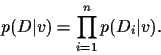
![$\displaystyle 2
\frac{{\rm Re}\left[\sum_{k=1}^N
\varphi_k^*(x_i)
\partial_{v(z)}\varphi_k(x_i)
\right]}
{\sum_{l=1}^N \vert\varphi_l(x_i)\vert^2}
.$](img129.gif)