


Next: Regression
Up: Adapting prior means
Previous: Density estimation
Contents
Unrestricted variation
To get a first understanding of the approach (432)
let us consider the extreme example of
completely unrestricted  -variations.
In that case the template function
-variations.
In that case the template function  itself
represents the hyperparameter.
(Such function hyperparameters or hyperfields
are also discussed in Sect. 5.6.)
Then,
itself
represents the hyperparameter.
(Such function hyperparameters or hyperfields
are also discussed in Sect. 5.6.)
Then,
 and
Eq. (435) gives
and
Eq. (435) gives
 =
=  (which for invertible
  is solved uniquely by
  ),
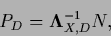
resulting according to Eq. (229) in
),
resulting according to Eq. (229) in
 |
(441) |
The case of a completely free prior mean
is therefore equivalent to a situation without prior.
Indeed, for invertible
 ,
projection of Eq. (436) into the
,
projection of Eq. (436) into the  -data space
by
-data space
by  of Eq. (260)
yields
of Eq. (260)
yields
 |
(442) |
where
 =
=
 is invertible
and
is invertible
and
 .
Thus for
.
Thus for  for which
  are available
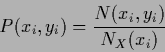 |
(443) |
is concentrated on the data points.
Comparing this with solutions of Eq. (228),
for  = fixed,
we see that adaptive means tend to lower the influence
of prior terms.
= fixed,
we see that adaptive means tend to lower the influence
of prior terms.
Next: Regression
Up: Adapting prior means
Previous: Density estimation
Contents
Joerg_Lemm
2001-01-21