Density estimation

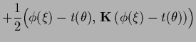
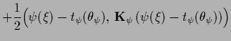
The general case with adaptive means for Gaussian prior factors and hyperparameter energy $E_\theta$ yields an error functional

$$E_{\theta,\phi} = -(\ln P(\phi),\,N) +\frac{1}{2} \Big(\phi-... ...}\,(\phi-t(\theta))\Big) + (P(\phi),\, \Lambda_X )+ E_\theta .$$ (432)

Defining

$${\bf t}^\prime (l;x,y) = \frac{\partial t(x,y;\theta)}{\partial \theta_l} ,$$ (433)

the stationarity equations of (432) obtained from the functional derivatives with respect to $\phi$ and hyperparameters $\theta$ become

$${{\bf K}}(\phi-t) = {\bf P}^\prime(\phi) {\bf P}^{-1}(\phi) N - {\bf P}^\prime (\phi) \Lambda_X ,$$ (434)

$${\bf t}^\prime {{\bf K}} (\phi-t) = E_{\theta}^\prime .$$ (435)

Inserting Eq. (434) in Eq. (435) gives

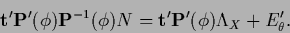$${\bf t}^\prime{\bf P}^\prime (\phi) {\bf P}^{-1}(\phi) N = ... ... t}^\prime{\bf P}^\prime(\phi) \Lambda_X +E_{\theta}^\prime .$$ (436)

Eq.(436) becomes equivalent to the parametric stationarity equation (356) with vanishing prior term in the deterministic limit of vanishing prior covariances ${\bf K}^{-1}$, i.e., under the assumption $\phi=t(\theta)$, and for vanishing $E_\theta^\prime$. Furthermore, a non-vanishing prior term in (356) can be identified with the term $E_\theta$. This shows, that parametric methods can be considered as deterministic limits of (prior mean) hyperparameter approaches. In particular, a parametric solution can thus serve as reference template $t$, to be used within a specific prior factor. Similarly, such a parametric solution is a natural initial guess for a nonparametric $\phi$ when solving a stationarity equation by iteration.

If working with parameterized $\phi(\xi)$ extra prior terms Gaussian in some function $\psi(\xi)$ can be included as discussed in Section 4.2. Then, analogously to templates $t$ for $\phi$, also parameter templates $t_\psi$ can be made adaptive with hyperparameters $\theta_\psi$. Furthermore, prior terms $E_\theta$ and $E_{\theta_\psi}$ for the hyperparameters $\theta$, $\theta_\psi$ can be added. Including such additional error terms yields

$$E_{\theta,\theta_\psi,\phi(\xi),\psi(\xi)} = -(\ln P(\,\phi(\xi)\,),\,N) + (P(\,\phi(\xi)\,),\, \Lambda_X )$$

$$+\frac{1}{2} \Big(\phi(\xi)-t(\theta) ,\,{{\bf K}}\,(\phi(\xi)-t(\theta))\Big)$$

$$+\frac{1}{2} \Big(\psi(\xi)-t_\psi(\theta_\psi), \,{{\bf K}}_\psi\,(\psi(\xi)-t_\psi(\theta_\psi))\Big)$$

$$+E_{\theta} + E_{\theta_\psi} ,$$ (437)

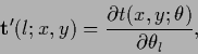
and Eqs.(434) and (434) change to

$$\Phi^\prime {{\bf K}}(\phi-t) +\Psi^\prime {{\bf K}}_\psi (\psi-t_\psi) = {\bf P}_\xi^\prime {\bf P}^{-1}N - {\bf P}_\xi^\prime \Lambda_X ,$$ (438)

$${\bf t}^\prime {{\bf K}} (\phi-t) = E_{\theta}^\prime ,$$ (439)

$${\bf t}_\psi^\prime {{\bf K}}_\psi (\psi-t_\psi) = E_{\theta_\psi}^\prime,$$ (440)

where ${\bf t}_\psi^\prime$, $E_{\theta_\psi}^\prime$, $E_{\theta}^\prime$ , denote derivatives with respect to the parameters $\theta_\psi$ or $\theta$, respectively. Parameterizing $E_{\theta}$ and $E_{\theta_\psi}$ the process of introducing hyperparameters can be iterated.