Inverse quantum mechanics

Up to now we have formulated the learning problem in terms of a function $\phi$ having a simple, e.g., pointwise, relation to $P$. Nonlocalities in the relation between $\phi$ and $P$ was only due to the normalization condition, or, working with the distribution function, due to an integration. Inverse problems for quantum mechanical systems provide examples of more complicated, nonlocal relations between likelihoods $p(y\vert x,h)$ = $p(y\vert x,\phi)$ and the hidden variables $\phi$ the theory is formulated in. To show the flexibility of Bayesian Field Theory we will give in the following a short introduction to its application to inverse quantum mechanics. A more detailed discussion of inverse quantum problems including numerical applications can be found in [133,143,142,138,222].

The state of a quantum mechanical systems can be completely described by giving its density operator $\rho$. The density operator of a specific system depends on its preparation and its Hamiltonian, governing the time evolution of the system. The inverse problem of quantum mechanics consists in the reconstruction of $\rho$ from observational data. Typically, one studies systems with identical preparation but differing Hamiltonians. Consider for example Hamiltonians of the form ${\bf H} = {\bf T} + {\bf V}$, consisting of a kinetic energy part ${\bf T}$ and a potential ${\bf V}$. Assuming the kinetic energy to be fixed, the inverse problem is that of reconstructing the potential ${\bf V}$ from measurements. A local potential ${\bf V}(y,y^\prime )$ = $V(y)\delta (y-y^\prime )$ is specified by a function $V(y)$. Thus, for reconstructing a local potential it is the function $V(y)$ which determines the likelihood $p(y\vert x,h)$ = $p(y\vert{\bf X},\rho)$ = $p(y\vert{\bf X},V)$ = $P(\phi)$ and it is natural to formulate the prior in terms of the function $\phi$ = $V$. The possibilities of implementing prior information for $V$ are similar to those we discuss in this paper for general density estimation problems. It is the likelihood model where inverse quantum mechanics differs from general density estimation.

Measuring quantum systems the variable $x$ corresponds to a hermitian operator ${\bf X}$. The possible outcomes $y$ of measurements are given by the eigenvalues of ${\bf X}$, i.e.,

$${\bf X} \vert y> = y \vert y> ,$$ (338)

where $\vert y>$, with dual $<y\vert$, denotes the eigenfunction with eigenvalue $y$. (For the sake of simplicity we assume nondegenerate eigenvalues, the generalization to the degenerate case being straightforward.) Defining the projector

$$\Pi_{{\bf X},y} = \vert y\!><\!y\vert$$ (339)

the likelihood model of quantum mechanics is given by

$$p(y\vert x,\rho) = {\rm Tr} (\Pi_{{\bf X},y} \rho) .$$ (340)

In the simplest case, where the system is in a pure state, say the ground state $\varphi_0$ of ${\bf H}$ fulfilling

$${\bf H}\vert\varphi_0> = E_0\vert\varphi_0> ,$$ (341)

the density operator is

$$\rho = \rho^2 = \vert\varphi_0\!><\!\varphi_0\vert ,$$ (342)

and the likelihood (340) becomes

$$p(y\vert x,h) =p(y\vert{\bf X},\rho) = {\rm Tr} (\vert\varphi_0\!><\!\varphi_0\vert y><y\vert) = \vert\varphi_0(y)\vert^2 .$$ (343)

Other common choices for $\rho$ are shown in Table 4.

In contrast to ideal measurements on classical systems, quantum measurements change the state of the system. Thus, in case one is interested in repeated measurements for the same $\rho$, that density operator has to be prepared before each measurement. For a stationary state at finite temperature, for example, this can be achieved by waiting until the system is again in thermal equilibrium.

Table 4: The most common examples of density operators for quantum systems. In this table $\psi$ denotes an arbitrary pure state, $\varphi _i$ represents an eigenstate of Hamiltonian ${\bf H}$. The unitary time evolution operator for a time-independent Hamiltonian ${\bf H}$ is given by ${\bf U}$ = $e^{-i(t-t_0) {\bf H}}$. In scattering one imposes typically additional specific boundary conditions on the initial and final states.

	$\rho$
general pure state	$\vert\psi><\psi\vert$
stationary pure state	$\vert\varphi_i({\bf H}) ><\varphi_i({\bf H})\vert$
ground state	$\vert\varphi_0({\bf H})\vert><\varphi_0({\bf H})\vert$
time-dependent pure state	$\vert{\bf U}(t,t_0)\psi(t_0)><{\bf U}(t,t_0)\psi(t_0)\vert$
scattering	$\lim_{t\rightarrow\infty\atop t_0\rightarrow-\infty} \vert{\bf U}(t,t_0)\psi(t_0)><{\bf U}(t,t_0)\psi(t_0)\vert$
general mixture state	$\sum_k p(k) \;\vert\psi_k><\psi_k\vert$
stationary mixture state	$\sum_i p(i\vert{\bf H}) \;\vert\varphi_i ({\bf H}) ><\varphi_i ({\bf H}) \vert$
canonical ensemble	$({\rm Tr}\, e^{-\beta {\bf H}})^{-1} e^{-\beta {\bf H}}$

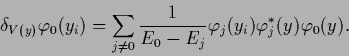
For a Maximum A Posteriori Approximation the functional derivative of the likelihood is needed. Thus, for reconstructing a local potential we have to calculate

$$\delta_{V(y)} p(y_i\vert{\bf X},V) .$$ (344)

To be specific, let us assume we measure particle coordinates, meaning we have chosen ${\bf X}$ to be the coordinate operator. For a system prepared in the ground state of its Hamiltonian ${\bf H}$, we then have to find,

$$\delta_{V(y)} \vert\varphi_0 (y_i)\vert^2 .$$ (345)

For that purpose, we take the functional derivative of Eq. (341), which yields

$$({\bf H}-E_0)\vert\delta_{V(y)} \varphi_0\!> = (\delta_{V(y)} {\bf H} -\delta_{V(y)} E_0)\vert\varphi_0\!> .$$ (346)

Projecting from the left by $<\!\varphi_0\vert$, using again Eq. (341) and the fact that for a local potential $\delta_{V(y)} {\bf H}(y^\prime,y^{\prime\prime})$ = $\delta (y-y^\prime)\delta(y^\prime-y^{\prime\prime})$, shows that

$$\delta_{V(y)} E_0 = <\!\varphi_0\vert\delta_{V(y)} {\bf H}\vert\varphi_0\!> = \vert\varphi_0(y)\vert^2 .$$ (347)

Choosing $<\!\varphi_0\vert\delta_{V(y)} \varphi_0\!>$ = 0 and inserting a complete basis of eigenfunctions $\vert\varphi_j\!>$ of ${\bf H}$, we end up with

$$\delta_{V(y)} \varphi_0 (y_i) = \sum_{j\ne 0} \frac{1}{E_0-E_j} \varphi_j (y_i) \varphi_j^* (y) \varphi_0 (y) .$$ (348)

From this the functional derivative of the quantum mechanical log-likelihood (345) corresponding to data point $y_i$ can be obtained easily,

$$\delta_{V(y)} \ln p(y_i\vert{\bf X},V) = 2 {\rm Re} \left( \varphi_0(y_i)^{-1} \delta_{V(y)} \varphi_0 (y_i)\right) .$$ (349)

The MAP equations for inverse quantum mechanics are obtained by including the functional derivatives of the prior term for $V$. In particular, for a Gaussian prior with mean $V_0$ and inverse covariance ${\bf K}_V$, acting in the space of potential functions $V(y)$, its negative logarithm, i.e., its prior error functional, reads

$$\frac{1}{2} \Big(V-V_0,\; {\bf K}_V \,(V-V_0)\Big) +\ln Z_V ,$$ (350)

with $Z_V$ being the $V$-independent constant normalizing the prior over $V$. Collecting likelihood and prior terms, the stationarity equation finally becomes

$$0= \sum_i \delta_{V(y)} \ln p(y_i\vert{\bf X},V) - {\bf K}_V \,(V-V_0) .$$ (351)

The Bayesian approach to inverse quantum problems is quite flexible and can be used for many different learning scenarios and quantum systems. By adapting Eq. (349), it can deal with measurements of different observables, for example, coordinates, momenta, energies, and with other density operators, describing, for example, time-dependent states or systems at finite temperature [143].

The treatment of bound state or scattering problems for quantum many-body systems requires additional approximations. Common are, for example, mean field methods, for bound state problems [55,197,27] as well as for scattering theory [78,27,140,141,130,131,223]. Referring to such mean field methods inverse quantum problems can also be treated for many-body systems [142].