Average energy

Using a standard Gaussian smoothness prior as in Eq. (34) with zero reference potential $v_0 \equiv 0$ (and, say, zero boundary conditions for $v$) leads to flat potentials for large smoothness factors $\lambda$. Especially in such cases it turned out to be useful to include besides smoothness also a priori information which determines the depth of the potential. One such possibility is to include information about the average energy

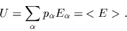$$U = \sum_\alpha p_\alpha E_\alpha =\, <E> .$$ (41)

We may remark, that for fixed boundary values of $v$ a certain average energy cannot be obtained by simply adding a constant to the potential. The average energy can, however, be set to a value $\kappa$ by including a Lagrange multiplier term

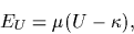$$E_U = \mu (U - \kappa) ,$$ (42)

Similarly, and technically sometimes easier, one can include noisy `energy data' of the form

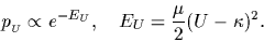$$p_{{}_{\scriptsize U}} %%p_U \propto e^{-E_U} ,\quad E_U = \frac{\mu}{2} (U - \kappa)^2 .$$ (43)

For $\mu\rightarrow\infty$ this results in $U\rightarrow\kappa$ so both approaches coincide.