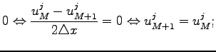
Next: Examples Up: Numerical solution Previous: Numerical solution
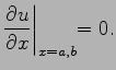
on the interval
| (2.23) |
Let us try to apply a simple explicit scheme (2.10) to Eq. (2.18). The discretization scheme reads
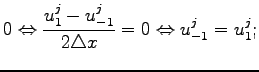
To the implementation of the second initial condition one needs again the virtual point ![]() ,
,
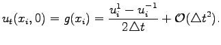
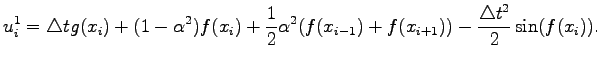
So, one can rewrite the last expression as
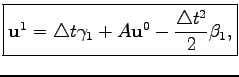
and the second time row can be calculated as
 |
(2.25) |
 |
 |
||
 |
 |
 |
(2.26) |
 and and |
|||
 |
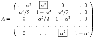
The boxed elements indicate the influence of periodic boundary conditions. Other time rows can also be written in the matrix form as
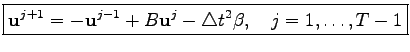 |
(2.27) |
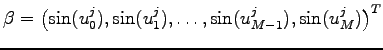
is a
Gurevich_Svetlana 2008-11-12