Complex, non-Gaussian prior factors, for example being multimodal, may be constructed or approximated by using mixtures of simpler prior components. In particular, it is convenient to use as components or ``building blocks'' Gaussian densities, as then many useful results obtained for Gaussian processes survive the generalization to mixture models [132,133,134,135,136]. We will therefore in the following discuss applications of mixtures of Gaussian priors. Other implementations of non-Gaussian priors will be discussed in Section 6.5.
In Section 5.1 we have seen that
hyperparameters label components of mixture densities.
Thus, if ![]() labels the components of a mixture model,
then
labels the components of a mixture model,
then ![]() can be seen as hyperparameter.
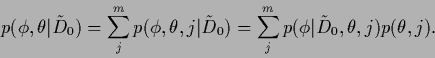
In Section 5
we have treated the corresponding hyperparameter integration
completely in saddle point approximation.
In this section we will assume the hyperparameters
can be seen as hyperparameter.
In Section 5
we have treated the corresponding hyperparameter integration
completely in saddle point approximation.
In this section we will assume the hyperparameters ![]() to be discrete and try to calculate
the corresponding summation exactly.
to be discrete and try to calculate
the corresponding summation exactly.
Hence, consider
a discrete hyperparameter ![]() ,
possibly in addition to continuous hyperparameters
,
possibly in addition to continuous hyperparameters ![]() .
In contrast to the
.
In contrast to the ![]() -integral
we aim now in treating the analogous sum over
-integral
we aim now in treating the analogous sum over ![]() exactly,
i.e., we want to study mixture models
exactly,
i.e., we want to study mixture models
 .
If the sum is reduced to a single term,
then
.
If the sum is reduced to a single term,
then
We already discussed shortly in Section 5.2 that,
in contrast to a product of probabilities or a sum of error terms
implementing a probabilistic AND of approximation conditions,
a sum over ![]() implements a probabilistic OR.
Those alternative approximation conditions will in the sequel
be represented by alternative templates
implements a probabilistic OR.
Those alternative approximation conditions will in the sequel
be represented by alternative templates ![]() and
inverse covariances
and
inverse covariances ![]() .
A prior (or posterior) density in form of a probabilistic OR means that
the optimal solution does not necessarily have to approximate
all but possibly only one of the
.
A prior (or posterior) density in form of a probabilistic OR means that
the optimal solution does not necessarily have to approximate
all but possibly only one of the ![]() (in a metric defined by
(in a metric defined by ![]() ).
For example, we may expect in an image reconstruction task
blue or brown eyes whereas a mixture
between blue and brown might not be as likely.
Prior mixture models are potentially useful for
).
For example, we may expect in an image reconstruction task
blue or brown eyes whereas a mixture
between blue and brown might not be as likely.
Prior mixture models are potentially useful for
For a discussion of possible applications of prior mixture models see also [132,133,134,135,136]. An application of prior mixture models to image completion can be found in [137].