This is the most widely used algorithm for cone beam tomography with the source running on a circle. It is well known that this inversion problem is highly unstable. But practical experience with the FDK formula is nevertheless quite encouraging.
The function which is sampled in cone beam tomography with the source on a circle is
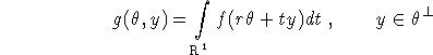
where ![]() is a direction vector in the
is a direction vector in the ![]() -plane,
-plane, ![]() .
. ![]() is the subspace orthogonal to
is the subspace orthogonal to ![]() , while
, while ![]() (see below) is the vector
(see below) is the vector ![]() perpendicular to
perpendicular to ![]() . As usual we assume f = 0 outside
. As usual we assume f = 0 outside ![]() where
where ![]() .
.
The FDK formula is an ingenious adaption of the 2D inversion formula of section 2.4 to 3D. Consider
the plane ![]() through
through ![]() and x which intersects
and x which intersects ![]() in a line
parallel to the
in a line
parallel to the ![]() -plane. Compute in this plane for each
-plane. Compute in this plane for each ![]() the
contribution to (2.14). Finally, integrate all these contributions over
the
contribution to (2.14). Finally, integrate all these contributions over ![]() , disregarding that those contributions come from different planes.
, disregarding that those contributions come from different planes.
The necessary computations are unpleasant, but the result is fairly simple. Based on (2.14),
where
![]()
and ![]() , z are coordinates in
, z are coordinates in ![]() , i.e.
, i.e. ![]() stands for
stands for ![]() with
with ![]() . The
implementation of (3.3) leads to a reconstruction algorithm of the filtered
backprojection type. The reconstructions computed with the FDK formula (3.3) are
- understandably - quite good for flat objects, i.e. if f is non-zero only close to the
. The
implementation of (3.3) leads to a reconstruction algorithm of the filtered
backprojection type. The reconstructions computed with the FDK formula (3.3) are
- understandably - quite good for flat objects, i.e. if f is non-zero only close to the ![]() -plane in which the source runs. If this is not the case then exact formula using
more data such as Grangeat's formula, see below, have to be used.
-plane in which the source runs. If this is not the case then exact formula using
more data such as Grangeat's formula, see below, have to be used.
