In 3D CT one reconstructes a from the values of
![]()
where v runs through the source curve V outside supp(a) and ![]() . Most reconstruction formulas make use of an intermediate function
. Most reconstruction formulas make use of an intermediate function
![]()
where h is homogeneous of degree -2 and a function F on ![]() derived from G by
derived from G by
![]()
The reconstruction formula then reads
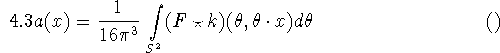
where the convolution with the 1D function k in the second argument. It can be shown that (4.1-3) is in fact a reconstruction formula provided that
![]()
For the proof we start out from
![]()
with the 3D Radon transform [49], hence ![]() . Then, (4.3) is compared with (2.4) for n = 3, i.e.
. Then, (4.3) is compared with (2.4) for n = 3, i.e.
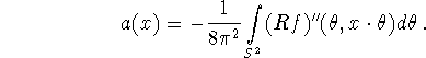
This coincides with (4.3) if (4.4) holds.
The simplest choice for h, k is ![]() ,
, ![]() . In this case, both
. In this case, both ![]() ,
, ![]() are local. We obtain Grangeat's inversion formula [19]
are local. We obtain Grangeat's inversion formula [19]
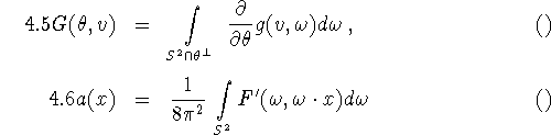
where ![]() is the derivative in direction
is the derivative in direction ![]() with respect to the second argument and
with respect to the second argument and ![]() is the partial derivative with respect to the second argument. In order to apply (4.5-6),
is the partial derivative with respect to the second argument. In order to apply (4.5-6), ![]() is needed for each plane
is needed for each plane ![]() meeting supp(a). Since F is obtained from G by means of (4.2) we need for each such plane
a source v in that plane. In view of (4.5) this means that g is available for a neighbourhood of the fan in that plane converging to the source v. This is Grangeat's completeness condition.
meeting supp(a). Since F is obtained from G by means of (4.2) we need for each such plane
a source v in that plane. In view of (4.5) this means that g is available for a neighbourhood of the fan in that plane converging to the source v. This is Grangeat's completeness condition.
The inversion formulas of Tuy [53], B. Smith [50] and Gelfand and Goncharov
[17] can be obtained by putting ![]() ,
, ![]() and
and ![]() ,
, ![]() , respectively [12]. These formulas are not as useful as Grangeat's formula since h is no longer local.
, respectively [12]. These formulas are not as useful as Grangeat's formula since h is no longer local.
In practice ![]() is measured on a detector plane
is measured on a detector plane ![]() where
where ![]() is the orthogonal projection of v onto
is the orthogonal projection of v onto ![]() . Putting
. Putting ![]() , (4.1) assumes the form
, (4.1) assumes the form
Introducing an orthogonal system ![]() in
in ![]() we obtain in the Grangeat case (4.5)
we obtain in the Grangeat case (4.5)
![]()
where ![]() , R is the 2D Radon transform and
, R is the 2D Radon transform and ![]() the gradient of
the gradient of ![]() . Thus Grangeat's formula can be implemented by computing line integrals in the detector plane, followed by a 3D backprojection (4.6). An implementation analogous to the filtered backprojection algorithm of 2D tomography can be found in [12].
. Thus Grangeat's formula can be implemented by computing line integrals in the detector plane, followed by a 3D backprojection (4.6). An implementation analogous to the filtered backprojection algorithm of 2D tomography can be found in [12].
In 3D emission CT, the requirements are quite different. In PET one puts the object into a vertical cylinder whose interior surface is covered by detectors. With such an arrangement one measures the X-ray transform for all lines joining two points on the mantle of the cylinder. In principle one could do the reconstruction layer by layer, using only horizontal lines in each layer. However, all the information contained in the oblique rays would be lost.
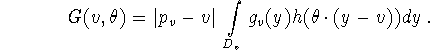
A formula which at least partially copes with this situation is
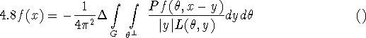
where ![]() is a spherical zone around the equator and
is a spherical zone around the equator and ![]() is the length of the intersection of G and the plane spanned by
is the length of the intersection of G and the plane spanned by ![]() , y [41]. With (4.8) one still has problems near the openings of the cylinder. More satisfactory reconstruction formulas based on the principle of the stationary phase have been given in [11].
, y [41]. With (4.8) one still has problems near the openings of the cylinder. More satisfactory reconstruction formulas based on the principle of the stationary phase have been given in [11].