Classical regularization functionals
consist of a sum of quadratic concepts.
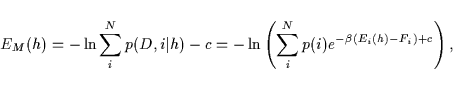
In a probabilistic interpretation
this corresponds to a combination by AND.
Typically, for example, a training data term AND a prior term
is approximated by ![]() .
The sum of quadratic concepts, however, is again a quadratic concept.
Analogously, a product of Gaussians is Gaussian.
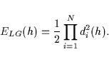
Straightforward calculation shows
that a sum of squared distances
.
The sum of quadratic concepts, however, is again a quadratic concept.
Analogously, a product of Gaussians is Gaussian.
Straightforward calculation shows
that a sum of squared distances ![]() with concept operators
with concept operators ![]() can be written
can be written
![]() ,
with squared distance
,
with squared distance
![]() template average
template average
![]() ,
,
![]() ,
,
![]() ,
and
,
and ![]() -independent minimal component energy
-independent minimal component energy
![]() ,
which has the structure of a variance up to a factor
,
which has the structure of a variance up to a factor ![]() .
The linear stationarity equation for a functional
.
The linear stationarity equation for a functional
![]() reads
reads
![]() .
For positive definite, i.e., invertible
.
For positive definite, i.e., invertible ![]() ,
this has solution
,
this has solution
![]() which can be solved in
a space with dimension smaller or equal to
which can be solved in
a space with dimension smaller or equal to ![]() [7,3]
.
Now let us present types of non-convex error functionals.
[7,3]
.
Now let us present types of non-convex error functionals.
Example:
Consider an image reconstruction task
where we expect the image of a face.
Thus, we may choose concepts with partial template functions
for eyes, nose and mouth
and require the reconstructed image to approximate
the given pixel data AND the eye, nose and mouth templates.
Typically, however, the constituents of a face
can appear in many different variations.
Eyes may be open OR closed,
blue OR brown but also
translated, scaled or otherwise deformed.
Such OR-like combinations of alternative concepts
are examples of non-convex prior knowledge.
In a probabilistic interpretation
of alternative concepts representing disjunct events
indexed by ![]() ,
this yields the mixture model
,
this yields the mixture model
Products are another possibility to implement OR-like structures
leading to technically convenient polynomial models